Quantum Matter Map

Quantum-matter problems connect composition and structure to collective states and measured signals. The path is rarely one-dimensional: the same Hamiltonian supports different phases, the same phase can arise from different microscopic models, and one experimental feature can have several explanations.

This map organizes the subject with two coordinates:

1. description layer — microscopic constituents, effective degrees of freedom, states, excitations, phases, and response;
2. experimental scale — the energy, length, momentum, time, temperature, and resolution at which a question is asked.

Use the Quantum Matter Overview for a quick entry decision. Use this map once a system or question has been chosen: it identifies missing assumptions and locates the canonical chapter for the next calculation. What Is Quantum Matter? owns the subject definition, while Quantum Matter supplies the full scientific synthesis. How to Use This Volume turns the map into goal- and depth-based learning routes.

How to Read the Map

Every concrete problem should be stated as a tuple:

$$\mathcal P = \left( \mathcal S, \mathcal H, \rho, \mathcal O, \mathcal R \right).$$

Here:

• $\mathcal S$ specifies the physical system and preparation;
• $\mathcal H$ is the microscopic or effective generator;
• $\rho$ is the state or ensemble;
• $\mathcal O$ is the observable or probe coupling;
• $\mathcal R$ specifies resolution, geometry, and the relevant limits.

Naming only a Hamiltonian leaves four parts unspecified. Naming only a material leaves all five partly implicit. A useful map must therefore route both from model to prediction and from measurement back to candidate models.

The forward direction

The forward problem is

$$\left( \mathcal S,\mathcal H,\rho,\mathcal O,\mathcal R \right) \longrightarrow p(\text{data}\mid\mathcal P).$$

It asks what a defined theory and preparation predict for a measurement, including uncertainty and finite resolution.

The inverse direction

The inverse problem is

$$\text{data} \longrightarrow \left\{ \text{models and parameters consistent with data} \right\}.$$

This arrow is generally many-to-one in reverse. It requires model comparison, calibration, and checks against complementary observables. The map is deliberately bidirectional because quantum-matter research alternates between these two tasks.

The Scale Ladder

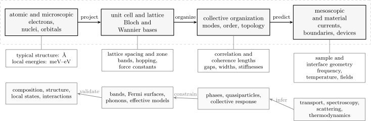
Descriptions are selected by scale and observable. Projection and organization move toward effective material theories; measurements constrain those theories in the reverse direction. The energy and length ranges overlap, so the diagram is a routing map rather than a claim of rigid scale separation.

The layers are not a sequence that must always be traversed from left to right. A sound-velocity problem may begin with elasticity. A core-level spectrum may require atomic multiplets. A quantized conductance problem may begin with channels and contacts. The correct entry point is the simplest layer that retains the information needed by the observable.

Layer 0: System and Preparation

Before writing a Hamiltonian, define what was made and how it was prepared.

Composition and structure

Record:

• chemical composition and stoichiometry;
• crystal structure, space group, and lattice parameters;
• dimensionality, thickness, stacking, and interfaces;
• defects, vacancies, substitutions, and disorder;
• strain, pressure, twist angle, and domain structure;
• substrate, encapsulation, contacts, and dielectric environment.

Nominal composition does not uniquely determine the electronic state. Oxygen content can set carrier density; strain can split orbitals; stacking can alter topology; disorder can create in-gap states; contacts can dominate a short device.

Thermodynamic and dynamical preparation

Specify temperature, magnetic field, electric field, pressure, gate voltage, illumination, cooling history, pulse sequence, and elapsed time. In driven systems, also specify frequency, amplitude, polarization, envelope, and coupling to reservoirs.

A state can depend on path:

$$\rho = \rho \left[ T(t),B(t),E(t),P(t),\ldots \right].$$

Hysteresis, metastability, glassiness, and prethermal behavior make the history more than a nuisance parameter.

Sample and instrument geometry

Current direction, surface orientation, polarization, scattering plane, contact layout, and boundary conditions select tensor components and matrix elements. “Conductivity” or “spectrum” is incomplete without this geometry.

Layer 1: Microscopic Ingredients

The microscopic description identifies the constituents and interactions from which lower-energy models are built.

Electronic and nuclear terms

A schematic electron–ion Hamiltonian is

$$H_{\mathrm{micro}} = T_{\mathrm e} +T_{\mathrm I} +V_{\mathrm{eI}} +V_{\mathrm{ee}} +V_{\mathrm{II}} +H_{\mathrm{rel}} +H_{\mathrm{ext}}.$$

Its material inputs include nuclear charges and masses, equilibrium geometry, electromagnetic environment, and external perturbations. Relativistic corrections can generate spin–orbit coupling in solids and magnetic anisotropy even when the dominant dynamics is nonrelativistic.

The Quantum Matter volume home states this hierarchy explicitly. Atomic and molecular electronic-structure foundations remain canonical in Atomic, Molecular, and Optical Physics.

Local states

Near each atom or molecular unit, useful labels may include:

• orbital character and occupancy;
• spin and total angular momentum;
• crystal-field or ligand-field multiplets;
• oxidation state and valence fluctuations;
• local phonon coordinates;
• electric and magnetic multipoles.

These labels are basis-dependent approximations, not tiny classical objects permanently attached to a site. Hybridization can spread an orbital across bonds, and strong spin–orbit coupling can make a total-angular-momentum multiplet more useful than separate spin and orbital labels.

Interaction inventory

List the interactions allowed at the scale of interest:

$$\left\{ t,\, U,\, V,\, J_{\mathrm H},\, \lambda_{\mathrm{SO}},\, g_{\mathrm{ep}},\, K,\, \Delta_{\mathrm{cf}},\, \ldots \right\}.$$

These can represent hopping, local and nonlocal Coulomb repulsion, Hund coupling, spin–orbit coupling, electron–phonon coupling, force constants, and crystal-field splitting.

The list is not yet a model. One must state the basis, operator definitions, range, signs, screening convention, and whether parameters are bare, downfolded, fitted, or renormalized.

Layer 2: Kinematics, Symmetry, and Constraints

Symmetry determines sectors, selection rules, protected degeneracies, allowed couplings, and candidate order parameters before a detailed solution is attempted.

Statistics and Hilbert space

Choose bosonic, fermionic, spin, rotor, constrained, or mixed degrees of freedom. State local occupancy rules and conserved quantities. A lattice with $L$ spinful fermion orbitals has a Fock-space dimension $4^L$ before symmetry reduction, so exploiting constraints is not optional in computation.

The canonical algebra lives in Identical Particles and Second Quantization.

Spatial symmetry

Translations produce crystal momentum; point-group operations constrain degeneracies and response tensors; nonsymmorphic symmetries can enforce band connectivity. A symmetry operation $g$ represented by $U_g$ obeys

$$U_gHU_g^{-1} = H$$

when it is exact. If $g$ maps momentum $\mathbf k$ to $g\mathbf k$, then a Bloch Hamiltonian satisfies

$$U_g(\mathbf k) H(\mathbf k) U_g^{-1}(\mathbf k) = H(g\mathbf k),$$

with basis-dependent sewing matrices and possible nonsymmorphic phases.

The abstract foundations are in Crystalline Symmetry Preview and Translations and Momentum.

Internal and discrete symmetries

Charge conservation, spin rotation, time reversal, particle–hole structure, inversion, mirror operations, and sublattice symmetries constrain phases and topological classifications. One must distinguish:

• exact microscopic symmetry;
• approximate symmetry valid below a scale;
• emergent symmetry of an infrared theory;
• symmetry broken explicitly by fields or disorder;
• symmetry broken spontaneously by the state.

Conservation and continuity

For a conserved density $n(\mathbf r,t)$ and current $\mathbf j$,

$$\frac{\partial n}{\partial t} + \boldsymbol\nabla\cdot\mathbf j = 0.$$

Continuity equations constrain low-frequency response and hydrodynamics. Lattice momentum, crystal momentum, mechanical momentum, and total momentum transferred to the environment must not be conflated.

Layer 3: Representation and Effective Model

The same physics can be represented in several bases. The representation should expose locality, symmetry, or the observable.

Real-space and localized bases

Atomic orbitals, Wannier functions, site spins, and bond variables make local interactions, defects, boundaries, and short-range hopping transparent. A generic lattice Hamiltonian is

$$H = \sum_{a,b} t_{ab}c_a^\dagger c_b + \frac{1}{2} \sum_{a,b,c,d} U_{abcd} c_a^\dagger c_b^\dagger c_d c_c + \cdots.$$

Localized bases are not unique. Gauge and orbital choices redistribute hopping range, interaction matrix elements, and position-operator structure while leaving physical predictions invariant when the basis is complete.

Reciprocal-space and band bases

Translation-invariant quadratic terms become block diagonal in crystal momentum:

$$H_0 = \sum_{\mathbf k} c_{\mathbf k}^\dagger h(\mathbf k) c_{\mathbf k}.$$

Diagonalizing the finite matrix $h(\mathbf k)$ gives band energies and eigenvectors. Energies alone are insufficient for optical, topological, and scattering questions because eigenvector geometry and matrix elements matter.

Collective and continuum variables

Long-wavelength descriptions use densities, currents, displacement fields, order parameters, phases, and gauge fields. Their coefficients encode integrated-out microscopic physics:

$$S_{\mathrm{eff}}[\phi] = \int dt\,d^dx\, \left[ \frac{\chi}{2}(\partial_t\phi)^2 - \frac{\rho_s}{2}(\boldsymbol\nabla\phi)^2 - V(\phi) + \cdots \right].$$

The field $\phi$ may describe a displacement, magnetic order, superconducting phase, or another collective coordinate. Its meaning, transformation law, and normalization must be defined.

Projection and downfolding

Let $P$ project onto retained states and $Q=1-P$. The exact energy-dependent effective operator has the schematic form

$$H_{\mathrm{eff}}(E) = PHP + PHQ \frac{1}{E-QHQ} QHP.$$

Approximating the resolvent produces low-energy Hamiltonians, superexchange, Schrieffer–Wolff transformations, and reduced-band models. Control depends on separation between retained and eliminated scales and on the observable.

The canonical derivation and error logic live in Effective Hamiltonians and Scale Separation.

When this problem decomposition leaves several retained descriptions plausible, Choosing a Model for Quantum Matter compares their adequacy for the declared observable and names the escalation test. This map owns the problem axes, not that candidate-model decision.

Layer 4: States, Excitations, and Phases

A Hamiltonian defines possible dynamics; a state specifies what is occupied, coherent, ordered, or out of equilibrium.

Ground and thermal states

At zero temperature, a nondegenerate ground state satisfies

$$H\lvert\Psi_0\rangle = E_0\lvert\Psi_0\rangle.$$

At equilibrium temperature $T$ and chemical potential $\mu$,

$$\rho = \frac{e^{-\beta(H-\mu N)}}{Z}, \qquad Z = \operatorname{Tr} e^{-\beta(H-\mu N)}.$$

Finite size, ensemble choice, boundary conditions, and order of limits can alter apparent degeneracy and response.

Elementary and emergent excitations

Relevant excitations include:

• electrons and holes in weakly interacting bands;
• quasiparticles with renormalized dispersion and lifetime;
• phonons, magnons, plasmons, and excitons;
• vortices, domain walls, solitons, and defects;
• fractionalized spinons, holons, and anyons;
• continua without a sharp particle interpretation.

The generic criteria for poles, widths, residues, and collective response live in Quasiparticles Overview and Collective Modes.

Phase organization

Candidate phases can be sorted by several nonexclusive structures:

Organizing structure	Examples	Defining diagnostics
filling and band structure	metal, semiconductor, band insulator	gap, Fermi surface, carrier response
spontaneous symmetry breaking	crystal, magnet, charge order	order parameter, correlations, collective modes
phase coherence	superfluid, superconductor	stiffness, flux response, vortices
topology of occupied states	Chern and topological insulators	invariant, gap, boundary and response
long-range entanglement	fractional Hall and spin-liquid phases	topological sectors, anyons, nonlocal structure
localization	Anderson or many-body localized regimes	transport, participation, level and dynamical diagnostics
nonequilibrium organization	Floquet, prethermal, driven steady states	protocol-dependent quasienergy or dynamical order

The rows overlap. A topological superconductor combines phase coherence with BdG topology; a magnetic topological insulator combines broken symmetry and band topology.

Layer 5: Observables and Probes

The final theory object must match what the instrument measures.

One-particle spectroscopy

Photoemission and tunneling constrain single-particle addition or removal spectra, filtered by occupation, matrix elements, surfaces, and resolution. The central object is a spectral function such as

$$A(\mathbf k,\omega) = - \frac{1}{\pi} \operatorname{Im} G^R(\mathbf k,\omega).$$

A band calculation predicts eigenvalues; an experiment records intensity. Relating them requires self-energy, matrix-element, final-state, surface, and resolution analysis.

Two-particle and collective probes

Neutron, x-ray, Raman, and optical probes couple to spin, charge, orbital, lattice, dipole, or current operators. A dynamical structure factor has the form

$$S_{OO}(\mathbf q,\omega) = \frac{1}{2\pi} \int dt\, e^{i\omega t} \langle O_{\mathbf q}(t) O_{-\mathbf q}(0) \rangle.$$

The operator $O$, polarization factors, form factors, and momentum coverage determine which fluctuations are visible.

Transport

Transport measures how currents respond to generalized forces. In linear response,

$$\langle J_a(\omega)\rangle = \sum_b \sigma_{ab}(\omega) E_b(\omega).$$

The dc limit can depend on the order of $\omega\to0$, $\mathbf q\to0$, thermodynamic, clean, and long-time limits. Contacts and geometry can dominate mesoscopic devices.

The canonical response derivation is Kubo Formula. Quantum matter owns the material mechanisms, tensor interpretation, and experimental comparison.

Thermodynamics and local probes

Heat capacity, magnetization, compressibility, thermal expansion, nuclear resonance, muon spin rotation, and local microscopy constrain derivatives of free energy or local correlation functions. They often distinguish bulk from surface effects and static from dynamic behavior.

No probe is universally superior. Reliability grows when observables sensitive to different operators support one consistent model.

The Ratio Map

Dimensionless ratios often reveal the correct regime more clearly than dimensional parameters.

Ratio	Compares	Typical interpretation
$T/T_F$	temperature to Fermi scale	degenerate or classical carrier statistics
$U/W$	interaction to bandwidth	itinerant, intermediate, or strongly correlated tendency
$\lambda_{\mathrm{SO}}/W$	spin–orbit to kinetic scale	weak perturbation or reorganized band multiplets
$\hbar\omega_D/E_F$	lattice to electronic scale	adiabatic hierarchy and vertex-correction relevance
$\Delta/k_BT$	gap to thermal broadening	whether a gap controls thermal response
$\Gamma/\Delta$	damping to gap or mode energy	sharp excitation or overdamped structure
$\ell_\phi/L$	coherence length to device size	coherent or incoherent transport regime
$k_F\ell$	wavelength to mean free path	clean metal, diffusive regime, localization proximity
$\xi/L$	correlation length to sample size	bulk scaling or finite-size crossover
$J_\perp/J_\parallel$	interlayer to intralayer coupling	three-dimensional or quasi-two-dimensional behavior

These ratios are diagnostics, not universal phase boundaries. Definitions and thresholds depend on model, dimension, and observable. For example, $U/W$ alone cannot classify a multi-orbital material with Hund coupling and charge-transfer physics.

Chapter Map

The volume is organized by the object that must be understood next.

Geometry and one-particle organization

This map selects the chapter from the broader problem tuple. When geometry and one-particle organization are next, enter the Lattices, Reciprocal Space, and Bloch Electrons gateway for its local dependency graph, then use the precise owners for Bravais lattices, reciprocal vectors, Brillouin zones, Bloch’s theorem, nearly free electrons, tight-binding models, Wannier functions, symmetry of Bloch states for little-group labels, protected degeneracies, and crossing compatibility, density of states, and Fermi surfaces.

Use Band Theory and Electronic Structure to route a declared band description, filling, gap or crossing question, and target observable. Continue to the Band Theory Overview for the band-to-many-body dictionary, metals, insulators, semiconductors, and semimetals for spectral classification, or effective masses for a validated local-extremum reduction. Wannier Functions separately owns the exact Bloch-subspace-to-localized-basis construction and its localization or obstruction audit.

Collective motion and response

Use the Lattice Vibrations and Collective Modes gateway to route among material lattice, carrier-dressing, charge-mode, and bound-pair questions. Phonons owns real-crystal dispersions, acoustic and optical branches, vibrational thermodynamics, and probe interpretation; the gateway supplies substantive fallbacks for the chapter’s planned electron–phonon, polaron, plasmon, and exciton branches.

Use Transport, Response, and Optics for Drude theory, Boltzmann transport, Kubo response, Hall effects, optical conductivity, thermoelectricity, sum rules, and hydrodynamic transport.

Ordered and topological phases

Use Magnetism and Spin Systems for moment and operator choice, exchange, ferro-, antiferro-, and ferrimagnetism, magnons, itinerant and impurity branches, spin–orbit coupling, spin transport, and Skyrmions and Magnetic Textures. Quantum spin liquids, fractionalization, and emergent gauge fields remain in the Strong Correlations and Emergence route below.

Use Superfluidity and Superconductivity for phenomenology, pairing, London electrodynamics and stiffness, BCS superconductivity theory, Ginzburg–Landau material phenomenology, the Josephson effect, vortices, and unconventional superconductivity.

After this map identifies a topological claim, enter Topological Quantum Matter to choose the band, Hall, superconducting, semimetal, interacting, boundary, transition, or computation branch. Use Topology in Quantum Matter for gapped-phase equivalence, protection assumptions, boundary logic, and the split between symmetry-protected and intrinsic order. Use Berry-Phase Polarization and Charge Pumping when the object is a crystalline polarization class or transported charge on a closed adiabatic cycle. Continue to Chern numbers in band theory for static occupied projectors, Hall response, and numerical invariants, then the integer quantum Hall effect, fractional quantum Hall effect, anyons and braiding, topological insulators, and topological superconductors before semimetals, crystalline topology, and broader interacting topological order.

Finite size, randomness, and strong coupling

Use What Is Mesoscopic Physics? for the independent confinement, mean-free-path, coherence, thermal, and contact scales. Continue to quantum coherence in conductors for dephasing and interference diagnostics, quantum wires for transverse subbands and one-dimensional density of states, conductance quantization for open-channel transmission, quantum dots for closed confinement and addition spectra, and Coulomb Blockade for orthodox tunneling thresholds and stability-diagram extraction.

Use Disorder, Localization, and Nonequilibrium Matter for impurity scattering, Anderson localization, disordered topology, driven phases, quench dynamics, and many-body localization caveats.

Use Strong Correlations and Emergence for interaction diagnostics, Mott insulators, Hubbard physics in materials, the projected t–J model, Kondo systems, heavy fermions, dynamical mean-field ideas, strange metals, quantum spin liquids, fractionalization, and emergent gauge fields.

Platforms, evidence, and tools

Use Low-Dimensional Quantum Matter to establish geometric versus effective dimension, confinement and crossover scales, dimensional state counting, and fluctuation constraints. Continue to Two-Dimensional Materials for monolayer crystals, dielectric environments, valleys, excitons, and device controls. Graphene is the first operator-level case study, following strain, masses, substrates, and interlayer tunnelling from a Dirac baseline into moiré matter. Transition-Metal Dichalcogenides is the complementary massive-valley case study, joining spin–valley locking and exciton spectroscopy to TMD moiré Hubbard and superconducting evidence. van der Waals Heterostructures then treats the whole stack as a device Hamiltonian, including interfaces, rotational alignment, encapsulation, gates, contacts, proximity, and vertical tunneling. Moiré Superlattices closes the scale hierarchy from reciprocal mismatch and reconstruction to mini Brillouin zones, minibands, filling, interactions, and analog simulation. Twisted Bilayer Graphene then follows one platform from the three-wave continuum Hamiltonian through the first magic regime, correlated states, superconductivity, and valley topology. Flat Bands provides the platform-independent account of compact localization, spectral flattening, projector geometry, Chern bands, and interaction amplification. Correlated Insulators in Moiré Systems then supplies the claim ladder from calibrated filling and bulk incompressibility to charge, flavor, and topological order. Moiré Superconductivity extends that evidence discipline to pairing, two-dimensional phase coherence, tunable domes, mechanism tests, and Josephson devices. Moiré Topology closes the route with topological minibands, Chern and QAH states, fractional Chern insulators, and topology–correlation competition.

2D Magnets and Ferroelectrics extends the route to anisotropy-stabilized magnetic order, layer parity, sliding polarization, and coupled ferroics. Engineered Heterostructures then compares transferred pairing, exchange, charge reconstruction, and cavity hybridization while separating constituent compatibility, interfacial transfer, and a genuinely new phase. Artificial Lattices and Designer Matter follows programmable graphs into quantum-dot, atomic, photonic, polaritonic, circuit, and assembled-electron implementations while keeping geometry, Hamiltonian, state, and phase claims distinct. Quantum Materials by Design closes the route by connecting target observables, Pareto screening, thermodynamic and kinetic evidence, synthesis, data-driven selection, property validation, and independent reproduction.

Use Probes, Devices, and Experiments for angle-resolved photoemission, tunneling, scattering, optics, transport, local probes, pressure, ultrafast methods, and uncertainty.

Use Computational Quantum Matter to turn a declared material claim into a routed workflow with model and parameter provenance, convergence tests, benchmarks, uncertainty, probe comparison, and a stopping rule.

Use Quantum Matter Frontiers and Open Problems only after the stable definitions and diagnostics are established; it freezes the claim, audits its evidence and alternatives, and routes durable physics separately from future living status. Use Quantum Matter Reference and Data to classify a lookup record, recover its conventions and provenance, and route it to the canonical physics owner and compact Reference handle.

Start from the Question

Question	First node	Next nodes
Why is this system metallic?	filling and band structure	interactions, disorder, Fermi surface, transport
Why is there a gap?	excitation type and symmetry	band, Mott, pairing, density-wave, topological possibilities
What carries current?	current operator and regime	quasiparticles, channels, hydrodynamics, contacts
What does this spectral peak represent?	probe operator and matrix element	pole, collective mode, bound state, continuum
Why is magnetic order absent?	moments, exchange, dimensionality	frustration, fluctuations, disorder, low ordering scale
Is the phase superconducting?	equilibrium electromagnetic response	stiffness, pairing, gap, vortices, phase-sensitive tests
Is the state topological?	gap and protection data	invariant, response, boundary, disorder and interaction stability
Which computation should I use?	observable and retained degrees	size, sign structure, entanglement, frequency and temperature

Starting from a named method reverses the proper order. Density-functional theory, tensor networks, Monte Carlo, and Green-function techniques answer different questions and fail in different ways.

Five Worked Routes

Route 1: a semiconductor optical edge

Observation: absorption rises above a threshold.

1. Establish crystal structure, temperature, polarization, thickness, and resolution.
2. Determine whether momentum conservation permits a direct transition or requires a phonon.
3. Build or obtain valence and conduction bands with orbital character.
4. Include dipole matrix elements, occupation factors, excitonic attraction, and lifetime broadening.
5. Compare the same model with transport activation or photoemission where available.

The optical threshold is not automatically the bare band gap. Excitons can lower it, phonons can enable indirect transitions, and disorder can add subgap absorption.

Route 2: anomalous Hall response

Observation: a transverse voltage appears without the ordinary field-linear Hall pattern.

1. Fix charge-sign, axis, field, and magnetization conventions.
2. Determine which symmetries permit an antisymmetric conductivity tensor.
3. Separate ordinary, intrinsic Berry-curvature, skew-scattering, and side-jump contributions.
4. Compare conductivity and resistivity scaling across temperature and disorder.
5. Test whether a validated band or interacting model reproduces magnitude and sign.

A nonzero Hall signal can indicate broken time-reversal symmetry, but it does not by itself establish a Chern insulator or quantized topology.

Route 3: missing order in a quantum magnet

Observation: no magnetic Bragg peak is found down to low temperature.

1. Confirm local moments and their energy scale with susceptibility, spectroscopy, or local probes.
2. Establish exchange geometry, anisotropy, and dimensionality.
3. Search for weak order, glassiness, structural disorder, and slow dynamics.
4. Characterize inelastic spectral weight and thermodynamic entropy.
5. Compare spin-liquid, valence-bond, disorder, and low-ordering-temperature models.

Absence of one signal is a constraint, not a complete phase identification.

Route 4: a superconducting tunneling gap

Observation: tunneling conductance is suppressed around zero bias with coherence-like peaks.

1. Establish bulk superconductivity using magnetic and transport response.
2. Model the normal-state density of states and tunneling matrix element.
3. Test gap anisotropy, temperature dependence, field response, and broadening.
4. Compare single-gap, multigap, nodal, pair-breaking, and competing-order descriptions.
5. Use phase-sensitive or momentum-sensitive probes for order-parameter symmetry.

A good fit to one broadened density-of-states formula does not uniquely determine the pairing mechanism.

Route 5: a correlated moiré insulator

Observation: resistance rises at an integer or fractional filling of a moiré band.

1. Characterize twist angle, strain, density calibration, displacement field, and inhomogeneity.
2. Compute or infer bandwidth, gaps to remote bands, topology, and screening.
3. Compare interaction, bandwidth, disorder, and temperature scales.
4. Distinguish symmetry-broken, Mott-like, Wigner-like, topological, and localization scenarios.
5. Test compressibility, activation, magnetism, optical response, and neighboring superconductivity with one consistent phase diagram.

The integer filling supplies a clue; it does not determine the mechanism.

Forward Models and Inference Models

A forward model predicts ideal observables from parameters $\boldsymbol\theta$:

$$\mathbf y_{\mathrm{ideal}} = \mathbf f(\boldsymbol\theta).$$

An experimental model includes calibration, resolution, nuisance parameters, and noise:

$$\mathbf y_{\mathrm{meas}} = \mathcal R \mathbf f(\boldsymbol\theta) + \mathbf b(\boldsymbol\eta) + \boldsymbol\epsilon.$$

$\mathcal R$ represents resolution and acceptance, $\mathbf b$ a background model, and $\boldsymbol\epsilon$ stochastic error. Parameters $\boldsymbol\eta$ may be physically uninteresting but essential for unbiased inference.

Identifiability

Parameters are identifiable only if distinct values produce distinguishable predictions under available measurements. A narrow frequency window may not separate mass renormalization from scattering rate; a momentum-integrated spectrum may not identify gap anisotropy.

Cross-validation across observables

A model gains credibility when one parameter set explains independent measurements. Parameters fitted separately to every curve can hide inconsistency.

Negative results

A null signal constrains a model only after sensitivity, coverage, and selection rules are quantified. Failure to observe a mode outside the instrument’s polarization or momentum window says little about its existence.

Computational Method Map

Choose methods by retained degrees of freedom and target observable.

Method family	Natural input	Strength	Central limitation
first-principles electronic structure	nuclei and crystal structure	realistic bands, energies, forces	functional and correlation approximations
tight binding and Wannier models	selected orbitals and matrix elements	symmetry, bands, boundaries, topology	truncation and parameter dependence
exact diagonalization	finite Hilbert-space Hamiltonian	unbiased spectra and correlations	exponential size growth
quantum Monte Carlo	sign-compatible path or operator weights	finite-temperature and ground-state statistics	sign problem and analytic continuation
tensor networks	local lattice Hamiltonian	entanglement-controlled low-dimensional states	bond dimension and dimensionality
dynamical mean-field methods	local self-energy embedding	strong local dynamics and spectra	nonlocal correlation treatment
Green-function perturbation	propagators and interaction vertices	spectra, response, diagrammatic control	expansion and self-consistency control
semiclassical and kinetic methods	bands, scattering, distribution functions	transport over broad scales	coherence and strong-correlation limits
continuum and hydrodynamic theory	symmetries, fields, constitutive data	universal long-wavelength response	microscopic coefficient input

Validation should include limiting cases, sum rules, conservation laws, finite-size or basis convergence, parameter uncertainty, and comparison with an independently solvable benchmark.

Canonical Boundaries

The map connects volumes without moving their canonical content.

• Fourier transforms, distributions, linear algebra, groups, topology, and numerical foundations live in Mathematical Toolkit.
• Identical particles, Fock space, occupation-number algebra, and entanglement definitions live in Composite Systems and Entanglement.
• Ensembles, correlation functions, generic lattice models, Kubo response, phases, and many-body computation live in Many-Body and Quantum Statistical Mechanics.
• Abstract translation, rotation, discrete symmetry, Berry geometry, and geometric phase live in Symmetry, Angular Momentum, and Spin.
• Approximation control, projection, perturbation theory, and scattering formalism live in Approximation and Semiclassical Methods.
• Open-system generators, baths, measurement backaction, and feedback live in Measurement and Open Systems.
• Atomic, molecular, spectroscopic, and light–matter building blocks live in Atomic, Molecular, and Optical Physics.

Quantum Matter owns the material specialization: crystalline bands, material collective modes, transport mechanisms, magnetic and superconducting phases, material topology, mesoscopic devices, disorder in solids, and probe-to-model inference.

Common Navigation Errors

Starting with the most sophisticated method

A more expensive calculation is not automatically closer to the observable. Begin by identifying the necessary degrees of freedom and accuracy.

Moving from a material name directly to a model

A compound can require different models at different energies and for different probes. State structure, filling, orbital content, and regime before selecting a canonical Hamiltonian.

Treating the hierarchy as strictly one-way

Experiments refine effective models, and emergent principles constrain microscopic possibilities. The map is an inference loop, not a reductionist conveyor belt.

Confusing a representation with a physical approximation

Changing from Bloch to Wannier basis can be exact within a chosen band subspace. Truncating bands, interaction range, or self-energy structure is an approximation. These operations must be reported separately.

Using one scale ratio as a phase label

$U/W$, $k_F\ell$, or $\Delta/k_BT$ can orient a calculation but cannot replace symmetry, filling, dimensionality, and response evidence.

Forgetting the probe operator

A mode can be present and invisible because of polarization, form factor, momentum coverage, or symmetry. Conversely, a peak can be produced by a matrix-element enhancement rather than a new density of states.

Promoting suggestive evidence to a unique assignment

Broad continua, zero-bias peaks, resistance anomalies, and boundary conduction have multiple causes. Use the map to identify discriminating observables.

Exercises

Exercise 1: complete the problem tuple

A paper states: “We simulated the Hubbard model and obtained an insulating state.” List the missing information needed to turn this into a defined material prediction.

Solution

At minimum, specify:

• lattice, dimension, size, and boundary conditions;
• orbital and spin content;
• hopping matrix elements, interaction terms, signs, and units;
• filling or chemical potential;
• temperature or state-preparation procedure;
• disorder and external fields;
• numerical method and convergence controls;
• the observable used to define “insulating”;
• frequency, momentum, and thermodynamic limits;
• mapping from model parameters to a material, if a material claim is intended.

An insulating charge gap, vanishing Drude weight, activated finite-temperature conductivity, and low compressibility are related but not identical diagnostics.

Exercise 2: choose a ratio

Select a dimensionless ratio for each question:

1. Are electrons thermally degenerate?
2. Is a mode spectrally sharp relative to its gap?
3. Can a device preserve phase coherence?
4. Are interaction and kinetic scales comparable?

Solution

1. $T/T_F$ compares temperature with the Fermi scale.
2. $\Gamma/\Delta$ or $\Gamma/\omega_0$ compares damping with the relevant excitation scale.
3. $\ell_\phi/L$ compares coherence length with device size.
4. $U/W$ compares interaction with bandwidth.

Each answer is only a first diagnostic. For example, $U/W$ does not include filling, Hund coupling, screening, or orbital degeneracy.

Exercise 3: exact basis change or approximation?

An isolated group of $M$ bands is transformed into $M$ Wannier orbitals per cell. The resulting Hamiltonian is then truncated to nearest-neighbor hopping and onsite interaction. Which step can be exact, and which is approximate?

Solution

A unitary transformation between a complete Bloch basis for the selected $M$-band subspace and $M$ Wannier orbitals per cell can be exact within that subspace, subject to topological and localization qualifications.

Selecting the $M$-band subspace already omits remote bands unless it is the full Hilbert space. Truncating hopping to nearest neighbors and interactions to onsite terms is an additional approximation. Its quality must be checked against discarded matrix elements and target observables.

Exercise 4: map an inverse problem

An optical conductivity shows a broad mid-infrared peak. Give four candidate mechanisms and one discriminating check for each.

Solution

Possible mechanisms include:

1. Interband transition: compare polarization, momentum-resolved bands, and selection rules.
2. Incoherent correlated spectral weight: test temperature and doping transfer against optical sum rules and photoemission.
3. Polaronic absorption: look for isotope, phonon, temperature, and lattice-coupling signatures.
4. Disorder or localization: vary disorder and compare low-frequency transport and localization length.
5. Collective mode: test field, momentum, symmetry, and linewidth behavior.

The same broad feature can contain several contributions, so a multi-component model may be necessary.

Exercise 5: order of limits

Explain why the two limits

$$\lim_{\omega\to0} \lim_{\mathbf q\to0} \chi(\mathbf q,\omega)$$

and

$$\lim_{\mathbf q\to0} \lim_{\omega\to0} \chi(\mathbf q,\omega)$$

need not agree. Give a physical interpretation.

Solution

Taking $\mathbf q\to0$ first describes a spatially uniform perturbation that can remain time dependent; taking $\omega\to0$ first describes a static perturbation with a long but finite wavelength. Conserved densities and collective transport respond differently in these protocols.

For example, a compressibility is a static equilibrium density response, while a uniform finite-frequency conductivity probes current dynamics. Continuity equations and relaxation determine whether spectral weight accumulates in a zero-frequency contribution. The observable must therefore specify the path to the origin in $(\mathbf q,\omega)$ space.

Exercise 6: design a cross-probe test

Design a minimal cross-probe program for deciding whether an apparent gap in a layered material is a band gap, a density-wave gap, or a superconducting gap.

Solution

Use:

1. momentum-resolved spectroscopy to locate which states gap and whether bands fold;
2. diffraction or a symmetry-sensitive local probe to test density-wave order;
3. magnetic screening and zero-resistance measurements to establish superconductivity;
4. tunneling or optics to compare gap scales and spectral-weight redistribution;
5. temperature, field, and polarization dependence to track the relevant order parameter and selection rules.

A band gap can persist without a thermodynamic transition, a density wave should introduce symmetry breaking or reconstruction, and a superconducting gap should accompany phase stiffness and characteristic field response. Coexistence is possible, so the analysis should allow more than one gap.

Connections

• From Quantum Mechanics to Materials works through one material-specific microscopic-to-effective provenance ledger; this page retains the reusable graph across systems, states, observables, and inverse problems.
• Quantum Matter provides the compact inference flow and full chapter route.
• What Is Quantum Matter? defines the subject and diagnostic hierarchy.
• 2D Magnets and Ferroelectrics follows reduced-dimensionality constraints into anisotropy-stabilized magnetism, layer-dependent order, switchable polarization, and coupled ferroic evidence.
• Engineered Heterostructures organizes cross-platform interface design around transferred interactions, parasitic channels, and phase-specific evidence.
• Artificial Lattices and Designer Matter organizes programmable lattice platforms around active-space, graph, parameter, state, open-system, detector, and prediction contracts.
• Quantum Materials by Design organizes inverse design around multiobjective targets, stability hierarchies, synthesis feedback, prospective tests, and reproducibility.
• How Quantum Matter Is Measured organizes experimental claims around forward models, instrumental resolution, surface and bulk weighting, equilibrium protocols, and orthogonal evidence.
• Transport Measurements follows electrical transport from four-terminal records through reversal, geometry, tensor, sweep-history, and uncertainty checks.
• Hall Measurements follows transverse records through signed-state reduction, carrier inference, multiband ambiguity, magnetic history, and quantum Hall validation.
• Quantum Oscillations follows oscillatory field records through inverse-field spectra, cyclotron masses, quantum lifetimes, orbit reconstruction, and phase cautions.
• Angle-Resolved Photoemission Spectroscopy follows photoelectron counts through energy–momentum maps, spectral line shapes, surface and matrix-element systematics, and correlation inference.
• Scanning Tunneling Microscopy and Spectroscopy follows junction current through feedback, topography, local spectra, setpoint effects, quasiparticle interference, gap maps, and atom manipulation.
• Neutron Scattering follows detector events through nuclear and magnetic cross sections, reciprocal-space kinematics, resolution, phonons, magnons, and continuum evidence.
• X-Ray Scattering follows photon counts through elastic structure refinement, resonant tensor contrast, charge-order inference, coherent phase retrieval, and inelastic energy-loss channels.
• Raman and Optical Spectroscopy follows scattered-light records through crystal tensors, phonon, magnon, and electronic channels, resonance, calibration, and thin-layer optical corrections.
• Terahertz and Infrared Probes follows power and field records through complex electrodynamics, carrier relaxation, superconducting gaps and stiffness, polar modes, multilayers, and time-domain uncertainty.
• Pump–Probe Spectroscopy follows calibrated nonequilibrium preparation through transient reflectivity, trARPES, coherent phonons, relaxation models, and phase-claim controls.
• Heat Capacity and Thermodynamics follows thermal records through calorimeter models, electronic and phonon components, transition anomalies, entropy, and low-temperature claim controls.
• Magnetic Susceptibility follows bulk moment records through unit, background, geometry, field-history, response-component, and phase-claim tests.
• Device Fabrication Concepts follows a material through contacts, gates, assembly, encapsulation, process disorder, cryogenic integration, and reproducibility controls.
• Data Interpretation and Pitfalls audits competing mechanisms, surface–bulk ambiguity, sample variation, inhomogeneity, contacts, topology, and hysteresis across probe families.
• Conventions for Quantum Matter fixes the lattice, Bloch, Berry, electromagnetic, spectral, and response contracts used by those routes.
• Charge and Spin Density Waves follows one symmetry-breaking route from finite-$\mathbf Q$ response through reconstruction, collective modes, and material evidence.
• Competing Orders compares exclusion, homogeneous coexistence, phase separation, and intertwined response using coupled-order phase diagrams and probe-aware evidence.
• Pair-Density Waves and Exotic Orders follows finite-momentum pair fields into composite charge, nematic, chiral, and higher-charge descendants, then audits material claims.
• Kondo Lattices follows a dense array of moments through Kondo–RKKY competition, lattice coherence, Fermi-volume counting, and Kondo-breakdown phase structures.
• Heavy Fermions follows local $f$ degrees of freedom into coherent quasiparticles, mass diagnostics, crossover scales, Fermi-volume inference, criticality, and superconductivity.
• Quantum Criticality follows controlled tuning into zero-temperature endpoints through fan reconstruction, scaling, thermodynamics, transport, and magnetic mechanism tests.
• Non-Fermi Liquids tests whether Landau quasiparticles fail and distinguishes momentum-selective, fractionalized, local, disordered, and holographic replacement theories.
• Strange Metals connects linear-$T$ transport to Planckian extraction caveats, optical and thermodynamic tests, and a cross-material mechanism ledger.
• Quantum Spin Liquids distinguishes material spin-liquid phases from weak order, trivial singlets, glasses, and disorder, then connects them to fractionalization and gauge evidence.
• Fractionalization defines deconfined excitation sectors and links one-dimensional spin–charge separation, fractional charge, symmetry quantum numbers, and material diagnostics.
• Emergent Gauge Fields follows microscopic constraints into Gauss laws, compact gauge dynamics, confinement or Higgs regimes, and gauge-invariant experimental evidence.
• Drude Theory is the first material transport benchmark and identifies when a single relaxation time is inadequate.
• Boltzmann Transport resolves the state-dependent distribution, collision operator, electrical response, and thermoelectric moments.
• Disorder in Quantum Matter supplies the source, ensemble, correlator, lifetime, and mean-free-path ledger needed before making a localization claim.
• Anderson Localization connects that statistical contract to eigenstate decay, bounded wave-packet spreading, typical transmission, dimensionality, and mobility edges.
• Weak Localization connects diffusive return paths to low-field magnetoconductance, dephasing fields, and weak-antilocalization channel tests.
• Scaling Theory of Localization connects those corrections to dimensionless-conductance flow, critical fixed points, exponent relations, and finite-size inference.
• Anderson Insulators connects localized states to bath-assisted hopping, Mott and Efros–Shklovskii laws, and independent parameter closure.
• Mobility Edges connects energy-resolved state character to three-dimensional Anderson criticality, transfer-matrix crossings, and probe resolution.
• Random Matrix Theory in Quantum Matter connects symmetry, spectral repulsion, quantum chaos, localization, and zero-dimensional topological classes.
• Glasses and Spin Glasses connects quenched frustration to overlap order, replica structure, aging response, and quantum-glass evidence.
• Many-Body Localization connects interacting disordered dynamics to platform controls, finite-window diagnostics, simulation limits, and active stability questions.
• Quantum Thermalization connects unitary many-body dynamics to subsystem observables, constrained ensembles, integrability controls, prethermal plateaus, and bath audits.
• Quenches connects parameter switches to finite-ramp calibration, energy injection, return amplitudes, propagating correlations, and ultrafast-material interpretation.
• Floquet Quantum Matter connects periodic controls to quasienergy observables, held-out effective-Hamiltonian tests, driven topology, and lifetime budgets across material platforms.
• Driven-Dissipative Matter connects sustained pump–loss balance to polariton fluids, output observables, finite-size transition evidence, and nonequilibrium field theory.
• Open Quantum Materials connects microscopic environments to complex poles, engineered dissipation, exceptional degeneracies, non-Hermitian boundaries, and metrological controls.
• Hall Effect shows how ordinary, multiband, anomalous, and quantized transverse signals support different levels of inference.
• What Is Mesoscopic Physics? connects finite geometry to confinement, coherent diffusion, thermal averaging, reservoirs, and sample-specific interference.
• Quantum Coherence in Conductors connects microscopic dephasing mechanisms to weak-localization fields, fluctuation correlations, ring harmonics, and saturation controls.
• Quantum Wires connects two-direction confinement to propagating subbands, Fermi points, threshold density of states, contacts, and interacting one-dimensional physics.
• Quantum Wells connects one-direction confinement to two-dimensional subbands, staircase density of states, heterostructures, and polarization-resolved optical transitions.
• Two-Dimensional Electron Gases connects interface occupation to density and interaction scales, disorder lifetimes, Hall quantization, spin–orbit response, and oxide-interface evidence.
• Graphene and Dirac Materials connects honeycomb-lattice bookkeeping to valley pseudospin, Berry-phase diagnostics, square-root Landau levels, and the moiré density scale.
• Quantum Dots connects finite-size confinement to orbital and charging spectra, spin filling, and optical excitons.
• Coulomb Blockade connects integer charge sectors to tunnel-junction rates, capacitance-controlled diamond edges, and single-electron-transistor operation.
• Single-Electron Devices connects controlled charge states to electrometry, event-resolved sensing, pumps, turnstiles, current standards, and device-level error budgets.
• Proximity and Andreev Physics connects electron–hole conversion to interface conductance, Andreev spectra, induced gaps, phase-biased weak links, and candidate Majorana hardware.
• Nanostructures for Quantum Technology connects nanoscale phenomena to functional primitives, measured error channels, process distributions, control infrastructure, and end-to-end task evidence.
• Quantum Point Contacts connects gate-defined bottlenecks to adiabatic modes, saddle calibration, partition noise, charge detection, and measurement backaction.
• Aharonov–Bohm Rings connects multiply connected geometry to flux periods, conductance harmonics, two-terminal phase rigidity, and ring-specific dephasing diagnostics.
• Universal Conductance Fluctuations connects coherent diffusion to sample-specific variance, magnetic and energy correlation scales, symmetry crossovers, and ensemble logic.
• Conductance Quantization connects one-dimensional mode thresholds to terminal conductance, degeneracy, contacts, and noise.
• Integer Quantum Hall Effect connects Hall plateaus to Landau filling, edge channels, localized bulk states, Chern response, and metrology.
• Fractional Quantum Hall Effect connects partial Landau-level filling to incompressible fluids, fractionalized quasiparticles, composite fermions, edges, and topological-order evidence.
• Topological Order connects ground-state topology and anyon data to modular matrices, $K$ matrices, entanglement, response, and evidence standards.
• Edge and Surface States compares boundary Hamiltonians, protection tests, hybridization gaps, and probe-specific evidence across topological phases.
• Bulk–Boundary Correspondence connects invariant mismatch to stable mode counting, anomaly inflow, domain walls, interacting alternatives, and strip numerics.
• Weyl and Dirac Semimetals connects bulk point crossings to Berry charge, Fermi arcs, crystalline protection, anomaly-related transport, and material claim tests.
• Symmetry-Protected Topological Phases connects symmetric gapped paths to projective edges, anomalous boundaries, interactions, stacking, and cohomological response.
• Magnetism and Spin Systems routes magnetic degrees of freedom, states, observables, and evidence to the precise material owner.
• Exchange Interactions connects orbital overlap, virtual charge states, mobile carriers, and Fermi-surface response to magnetic couplings.
• Ferromagnetism separates equilibrium uniform order from domain cancellation and nonequilibrium hysteresis.
• Antiferromagnetism connects compensated magnetic order to its ordering wavevector, sublattice structure, diffraction signatures, and field or current control.
• Ferrimagnetism connects ferrite site occupancy and unequal sublattice moments to compensation temperatures, collective modes, and devices.
• Spin Waves and Magnons supplies the material workflow from magnetic cell and local axes to bosonic modes, cross sections, resolution, and failure tests.
• Spintronics routes from spin generation and diffusion through magnetoresistive detection, charge–spin conversion, pumping, torque, and device-level tradeoffs.
• Skyrmions and Magnetic Textures separates topology, stability, dynamics, emergent electrodynamics, and experimental identification for walls, vortices, and skyrmions.
• Itinerant Magnetism routes from Fermi-surface susceptibility to exchange-split bands, spin-density waves, collective poles, and spin-fluctuation diagnostics.
• Stoner Criterion isolates the scalar uniform instability, its susceptibility enhancement, finite-temperature extension, and convention traps.
• Condensed Matter Roadmap supplies a prerequisite-first learning sequence.
• Math Needed for Quantum Matter routes mathematical preparation.
• Why Many-Body Physics Is Different develops the general emergence and scaling problem.
• Correlation Functions Overview explains the observables that connect states to experiments.
• Effective Hamiltonians in Quantum Matter specializes projection and matching logic.
• Reproducible Notebooks and Benchmark Problems give reusable computational validation standards.

References

Foundations and organization

1. N. W. Ashcroft and N. D. Mermin, Solid State Physics, Holt, Rinehart and Winston, 1976. The standard map from crystals and bands through phonons, response, and screening.
2. M. P. Marder, Condensed Matter Physics, 2nd ed., Wiley, 2010. A broad derivational treatment connecting microscopic models, elasticity, electrons, and phases.
3. P. Coleman, Introduction to Many-Body Physics, Cambridge University Press, 2015. Connects quasiparticles, response, magnetism, superconductivity, and strong-correlation models.
4. A. Altland and B. Simons, Condensed Matter Field Theory, 2nd ed., Cambridge University Press, 2010. Develops effective fields, Green functions, disorder, topology, and collective phenomena.
5. P. W. Anderson, “More Is Different,” Science 177, 393–396 (1972), doi:10.1126/science.177.4047.393. A foundational statement of scale-dependent organizing principles.

Quantum materials and inference

6. B. Keimer and J. E. Moore, “The Physics of Quantum Materials,” Nature Physics 13, 1045–1055 (2017), doi:10.1038/nphys4302. Reviews the interplay of correlations, entanglement, topology, and experimental control.
7. Y. Tokura, M. Kawasaki, and N. Nagaosa, “Emergent Functions of Quantum Materials,” Nature Physics 13, 1056–1068 (2017), doi:10.1038/nphys4274. Maps collective organization to experimentally useful material responses.
8. D. N. Basov, R. D. Averitt, D. van der Marel, M. Dressel, and K. Haule, “Electrodynamics of Correlated Electron Materials,” Reviews of Modern Physics 83, 471–541 (2011), doi:10.1103/RevModPhys.83.471. Demonstrates how optical observables, sum rules, and scale transfer constrain correlated models.
9. A. Damascelli, Z. Hussain, and Z.-X. Shen, “Angle-Resolved Photoemission Studies of the Cuprate Superconductors,” Reviews of Modern Physics 75, 473–541 (2003), doi:10.1103/RevModPhys.75.473. A detailed account of spectral functions, matrix elements, resolution, and inference.
10. A. Georges, G. Kotliar, W. Krauth, and M. J. Rozenberg, “Dynamical Mean-Field Theory of Strongly Correlated Fermion Systems and the Limit of Infinite Dimensions,” Reviews of Modern Physics 68, 13–125 (1996), doi:10.1103/RevModPhys.68.13. A canonical example of mapping a lattice problem to a self-consistent effective description.

Effective theories and computation

11. H. Georgi, “Effective Field Theory,” Annual Review of Nuclear and Particle Science 43, 209–252 (1993), doi:10.1146/annurev.ns.43.120193.001233. General principles of scale separation, operator organization, and matching.
12. E. Dagotto, “Correlated Electrons in High-Temperature Superconductors,” Reviews of Modern Physics 66, 763–840 (1994), doi:10.1103/RevModPhys.66.763. Shows how model selection, finite-size computation, and multiple observables interact in a difficult material problem.