Antiferromagnetism

Antiferromagnetism is magnetic order whose leading order parameter varies within the chemical unit cell or at a nonzero ordering wavevector. In the simplest collinear Néel state, two equivalent sublattices carry equal and opposite moments:

$$\mathbf M_0, \qquad -\mathbf M_0.$$

The ideal bulk uniform magnetization therefore vanishes even though each sublattice is ordered. This compensation is why ordinary magnetometry can miss an antiferromagnet and why diffraction, local probes, and symmetry-resolved measurements are central.

Antiferromagnetism is broader than the two-sublattice picture. Magnetic structures can be collinear or noncollinear, commensurate or incommensurate, localized-moment or itinerant, and single-$\mathbf Q$ or multi-$\mathbf Q$. Some antiferromagnets cant and acquire a small uniform moment; some remain metallic; some have strong antiferromagnetic correlations but no ordered phase. “Antiparallel neighboring spins” is therefore a useful motif, not a complete definition.

This page owns antiferromagnetism as a material phase: Néel order, sublattices and magnetic unit cells, ordering temperatures, field response, frustration, quantum fluctuations, experiments, and spintronic interpretation. Order Parameters owns the general source-selected definition, Heisenberg Model owns canonical lattice-model results, Magnons owns spin-wave quantization, and Exchange Interactions owns microscopic coupling pathways.

Required background. Exchange Interactions supplies material coupling signs, the Heisenberg Model supplies the lattice-spin convention, and Order Parameters supplies finite-wavevector source selection.

Helpful background. Ferromagnetism provides the uniform-order and domain contrast used throughout.

Néel Order Is Finite-Wavevector Order

Let a bipartite lattice be divided into sublattices $A$ and $B$, and define

$$\eta_i = \begin{cases} +1, &i\in A, \\[4pt] -1, &i\in B. \end{cases}$$

An ideal collinear Néel state has

$$\left\langle \mathbf s_i \right\rangle = \eta_i m_s\mathbf n,$$

where $m_s$ is the ordered spin per site and $\mathbf n$ is a unit vector specifying the Néel-axis orientation. The uniform spin average is zero when the two sublattices are equivalent, while the staggered average is nonzero:

$$\frac{1}{N} \sum_i \left\langle \mathbf s_i \right\rangle = \mathbf0, \qquad \frac{1}{N} \sum_i \eta_i \left\langle \mathbf s_i \right\rangle = m_s\mathbf n.$$

If an ordering wavevector $\mathbf Q_{\mathrm{AF}}$ satisfies

$$e^{i\mathbf Q_{\mathrm{AF}}\cdot\mathbf r_i} = \eta_i,$$

then the same order is the spin Fourier component at $\mathbf Q_{\mathrm{AF}}$. For a one-dimensional chain,

$$Q_{\mathrm{AF}} = \frac{\pi}{a},$$

and for the nearest-neighbor square lattice,

$$\mathbf Q_{\mathrm{AF}} = \left( \frac{\pi}{a}, \frac{\pi}{a} \right).$$

Wavevectors are defined modulo a chemical reciprocal-lattice vector. Crystallographic papers often quote them in reciprocal-lattice units, so the numerical coordinates depend on the chosen conventional cell.

Uniform and staggered variables

For two sublattice magnetization densities $\mathbf M_A$ and $\mathbf M_B$, a convenient convention is

$$\mathbf M = \frac{ \mathbf M_A+\mathbf M_B }{2}, \qquad \mathbf L = \frac{ \mathbf M_A-\mathbf M_B }{2}.$$

Here $\mathbf M$ is the uniform component and $\mathbf L$ is the Néel or staggered component. Other sources omit the factors of $1/2$; numerical comparisons require checking that normalization.

The inverse relations are

$$\mathbf M_A = \mathbf M+\mathbf L, \qquad \mathbf M_B = \mathbf M-\mathbf L.$$

If the two sublattice moments have equal fixed magnitude $M_0$, then

$$\mathbf M\cdot\mathbf L = 0, \qquad M^2+L^2 = M_0^2.$$

The ideal compensated state has $\mathbf M=\mathbf0$ and $\mathbf L=M_0\mathbf n$. A field-induced canting moment changes $\mathbf M$ without erasing $\mathbf L$.

The selecting source is staggered

A uniform magnetic field couples directly to $\mathbf M$, not to $\mathbf L$. The source conjugate to Néel order alternates between sublattices:

$$\Delta H_s = - \sum_i \eta_i \mathbf h_s\cdot\mathbf s_i.$$

The source-selected order parameter is

$$\mathbf m_s = \lim_{\mathbf h_s\to\mathbf0^+} \lim_{V\to\infty} \frac{1}{N} \sum_i \eta_i \left\langle \mathbf s_i \right\rangle_{\mathbf h_s}.$$

The thermodynamic limit comes first. A finite isotropic antiferromagnet can have a total-spin-singlet ground state and hence zero one-point staggered magnetization, while its correlations and low-lying spectrum already contain the approach to Néel order.

Correlation and Diffraction Diagnostics

The equal-time spin structure factor is

$$S(\mathbf q) = \frac{1}{N} \sum_{i,j} e^{i\mathbf q\cdot(\mathbf r_i-\mathbf r_j)} \left\langle \mathbf s_i\cdot\mathbf s_j \right\rangle.$$

With this normalization, true Néel long-range order gives

$$S(\mathbf Q_{\mathrm{AF}}) \sim N m_s^2$$

as $N\to\infty$. A large but subextensive peak can instead represent a long finite correlation length. The finite-size test is the scaled quantity

$$\frac{ S(\mathbf Q_{\mathrm{AF}}) }{N},$$

not merely whether the peak is visually prominent.

Elastic magnetic neutron diffraction measures a transverse magnetic structure factor. Schematically,

$$\mathbf F_M(\mathbf K) = \sum_j f_j(\mathbf K) e^{i\mathbf K\cdot\mathbf r_j} \left[ \mathbf M_j - \widehat{\mathbf K} \left( \widehat{\mathbf K}\cdot\mathbf M_j \right) \right],$$

and

$$I_M(\mathbf K) \propto \left| \mathbf F_M(\mathbf K) \right|^2.$$

The magnetic form factor $f_j$ reflects the spatial distribution of the magnetic electrons. The transverse projection means moments parallel to $\mathbf K$ do not contribute to that reflection.

For a commensurate antiferromagnet, new magnetic Bragg peaks can appear at

$$\mathbf K = \mathbf G \pm \mathbf Q_{\mathrm{AF}},$$

where $\mathbf G$ is a chemical reciprocal-lattice vector. If $\mathbf Q_{\mathrm{AF}}$ is itself equivalent to a structural reciprocal vector in the chosen cell, magnetic intensity may overlap nuclear peaks; polarization analysis, temperature dependence, and symmetry refinement are then needed.

Sublattices and the Magnetic Unit Cell

A graph is bipartite if its sites can be colored $A$ and $B$ so every relevant bond joins opposite colors. Nearest-neighbor square, honeycomb, and simple-cubic lattices are bipartite. A triangle is not: any two-coloring leaves one bond connecting equal colors.

On a bipartite crystal, a primitive chemical translation can interchange $A$ and $B$. The Néel state then has a larger magnetic unit cell than the chemical cell. A one-site translation changes

$$\mathbf n \longrightarrow -\mathbf n.$$

Time reversal also changes $\mathbf n\to-\mathbf n$. Each symmetry can be broken while their product remains a symmetry of a collinear antiferromagnetic state. Spin–orbit coupling and the actual crystallographic operation determine the full magnetic space group.

The orientations $\mathbf n$ and $-\mathbf n$ should not be identified casually. In a bipartite crystal they are distinct antiphase domains related by a broken translation or by time reversal, even though many bulk observables are even in $\mathbf n$. Whether a coarse-grained theory can treat the axis as director-like depends on which lattice and domain information has been integrated out.

Beyond two sublattices

The defining structure may require:

• three sublattices for $120^\circ$ triangular order;
• four or more sublattices for complex commensurate structures;
• an incommensurate phase $e^{i\mathbf Q\cdot\mathbf r}$ for spirals or spin-density waves;
• several symmetry-related wavevectors for multi-$\mathbf Q$ order;
• coupled spin, orbital, charge, or structural order parameters.

“Néel order” is most precise for a simple staggered collinear pattern. “Antiferromagnetic order” includes the wider family whose leading uniform moment is absent or secondary.

Exchange Selects the Ordering Wavevector

Use the exchange convention

$$H_{\mathrm{ex}} = \sum_{i<j} J_{ij} \mathbf s_i\cdot\mathbf s_j,$$

so $J_{ij}>0$ favors antiparallel bond correlations. For translation-invariant couplings, define

$$J(\mathbf q) = \sum_j J_{ij} e^{i\mathbf q\cdot(\mathbf r_j-\mathbf r_i)}.$$

At the classical or molecular-field level, the preferred ordering wavevector minimizes $J(\mathbf q)$. A nearest-neighbor bipartite antiferromagnet has its minimum at $\mathbf Q_{\mathrm{AF}}$, but competing further-neighbor interactions can move the minimum, create several minima, or select an incommensurate state.

A positive nearest-neighbor $J$ therefore establishes an antiferromagnetic bond tendency, not a theorem that the material has Néel order. Dimensionality, frustration, quantum fluctuations, anisotropy, disorder, itinerancy, and competing phases still decide the thermodynamic state.

Mean-field Néel temperature

For spin $S$, molecular-field theory gives a mode-dependent instability condition. If $\mathbf Q$ minimizes $J(\mathbf q)$,

$$k_{\mathrm B} T_N^{\mathrm{MF}} = - \frac{ S(S+1) }{3} J(\mathbf Q).$$

For nearest-neighbor exchange $J>0$ on a bipartite lattice with coordination $z$,

$$J(\mathbf0) = zJ, \qquad J(\mathbf Q_{\mathrm{AF}}) = -zJ,$$

and hence

$$k_{\mathrm B} T_N^{\mathrm{MF}} = \frac{ zJS(S+1) }{3}.$$

The high-temperature uniform susceptibility has Curie–Weiss form,

$$\chi = \frac{C}{ T-\Theta_{\mathrm{CW}} },$$

with

$$k_{\mathrm B} \Theta_{\mathrm{CW}} = - \frac{ S(S+1) }{3} J(\mathbf0).$$

Thus the simple nearest-neighbor mean-field model gives

$$\Theta_{\mathrm{CW}} = -T_N^{\mathrm{MF}}.$$

In a real material, $T_N$ and $|\Theta_{\mathrm{CW}}|$ need not agree. Short-range correlations, reduced dimensionality, frustration, itinerant fluctuations, disorder, and multiple exchanges can suppress or reshape the transition. A negative Weiss temperature is evidence for dominant antiferromagnetic correlations, not proof of a particular ordered structure.

Field Response, Canting, and Spin Flop

Compensation does not mean that an antiferromagnet cannot respond to a uniform field. The field cants the sublattice moments and produces a small $\mathbf M$ while the much larger staggered component remains.

A useful long-wavelength free-energy density is

$$\begin{aligned} f[\mathbf n,\mathbf M] ={}& \frac{M^2}{ 2\chi_\perp } + \frac{\rho_s}{2} \left| \boldsymbol\nabla\mathbf n \right|^2 \\ &+ \frac{K}{2} \left( 1-n_z^2 \right) - \mathbf h\cdot\mathbf M, \end{aligned}$$

subject to

$$\mathbf n^2 = 1, \qquad \mathbf n\cdot\mathbf M = 0.$$

Here $\mathbf h$ is the uniform source in the same energy-density convention as $\mathbf M$, $\chi_\perp$ is the transverse susceptibility, $\rho_s$ is spin stiffness, and $K>0$ gives an easy $z$ axis.

Minimizing over $\mathbf M$ gives

$$\mathbf M = \chi_\perp \left[ \mathbf h - \mathbf n \left( \mathbf n\cdot\mathbf h \right) \right].$$

The field gains energy most efficiently when $\mathbf n\perp\mathbf h$. For $\mathbf h=h\widehat{\mathbf z}$, compare:

$$f_{\parallel} = 0$$

for $\mathbf n\parallel\widehat{\mathbf z}$, and

$$f_{\perp} = \frac{K}{2} - \frac{ \chi_\perp h^2 }{2}$$

for $\mathbf n\perp\widehat{\mathbf z}$. In this minimal model, the ideal spin-flop scale is

$$h_{\mathrm{sf}} = \sqrt{ \frac{K}{ \chi_\perp } }.$$

Exchange-field notation often writes the same scale as $H_{\mathrm{sf}}\simeq\sqrt{2H_EH_A}$ when the anisotropy field $H_A$ is much smaller than the exchange field $H_E$. Factors depend on how those fields, sublattice moments, and SI units are defined.

The minimal formula omits longitudinal susceptibility, higher anisotropies, domains, magnetoelastic coupling, and the eventual saturation transition. Real spin-flop transitions can be rounded, split, hysteretic, or replaced by continuous rotation.

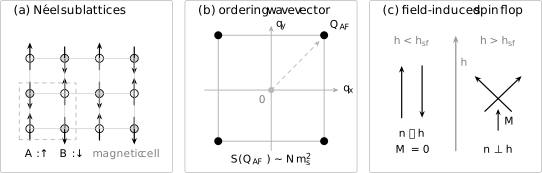
A collinear bipartite antiferromagnet alternates $A$ and $B$ moments, enlarging the magnetic periodicity. Its static structure factor is extensive at $\mathbf Q_{\mathrm{AF}}$, not at $\mathbf q=\mathbf0$. An easy-axis field can drive a spin-flop state in which the Néel vector turns transverse while both sublattices cant to produce a small uniform $\mathbf M$.

Weak ferromagnetism from antisymmetric exchange

The Dzyaloshinskii–Moriya interaction

$$H_{\mathrm{DM}} = \sum_{i<j} \mathbf D_{ij}\cdot \left( \mathbf s_i\times\mathbf s_j \right)$$

can cant otherwise antiparallel moments. At the schematic two-sublattice level,

$$\mathbf M \propto \frac{ \mathbf D\times\mathbf L }{J}.$$

The proportionality and sign depend on bond geometry and normalization. Such a canted antiferromagnet has primary staggered order and a secondary weak uniform moment. It is not a ferrimagnet, whose net moment comes from unequal opposing sublattice moments. Magnetic Anisotropy places this coupling in the full crystal, shape, and texture energy ledger.

Antiferromagnetic Domains

An antiferromagnet can have domains even when its external stray field is tiny. Distinct domain labels include:

• orientation domains, with different easy-axis or easy-plane directions;
• antiphase domains, related by $\mathbf n\to-\mathbf n$;
• wavevector domains, choosing different symmetry-related $\mathbf Q$ vectors;
• chirality domains in noncollinear structures;
• coupled structural, ferroelectric, or magnetoelastic domains.

Because a compensated bulk antiferromagnet has little magnetostatic energy, domain selection is often governed by crystalline anisotropy, magnetoelastic strain, defects, surfaces, exchange bias, and cooling history rather than the flux-closure balance familiar from ferromagnets.

Surfaces and interfaces can be uncompensated even when the bulk is compensated. A measured interfacial moment, exchange-bias shift, or local stray field therefore does not automatically represent the bulk uniform magnetization.

Spin Waves

Antiferromagnetic spin waves are collective oscillations of the coupled sublattices. For the nearest-neighbor bipartite Heisenberg model,

$$H = J \sum_{\langle i,j\rangle} \mathbf s_i\cdot\mathbf s_j, \qquad J>0,$$

linear spin-wave theory gives

$$\hbar\omega_{\mathbf k} = zJS \sqrt{ 1- \left| \gamma_{\mathbf k} \right|^2 },$$

where

$$\gamma_{\mathbf k} = \frac{1}{z} \sum_{\boldsymbol\delta} e^{i\mathbf k\cdot\boldsymbol\delta}$$

and $\boldsymbol\delta$ runs over nearest-neighbor vectors.

For the square lattice,

$$\gamma_{\mathbf k} = \frac12 \left[ \cos(k_xa) + \cos(k_ya) \right].$$

Near a gapless point, the dispersion is linear:

$$\hbar\omega \simeq \hbar c |\mathbf q|.$$

At the linear-spin-wave level for the square lattice,

$$c = \frac{ 2\sqrt2\,JSa }{\hbar}.$$

Momentum can be described in either the chemical Brillouin zone or the reduced magnetic Brillouin zone. Apparent duplication of gapless points must be interpreted with that folding convention.

Two type-A modes

An isotropic collinear antiferromagnet breaks

$$SO(3) \longrightarrow SO(2).$$

There are two broken spin generators. Unlike a ferromagnet, their commutator has no uniform magnetization expectation value in the compensated state. The two transverse coordinates therefore produce two type-A Goldstone polarizations with linear dispersion. Anisotropy, field, dipolar coupling, spin–orbit coupling, and intersublattice asymmetry can split or gap them.

Zero-point reduction

The classical Néel product state is not an eigenstate of an isotropic antiferromagnetic bond because

$$\mathbf s_i\cdot\mathbf s_j = s_i^zs_j^z + \frac12 \left( s_i^+s_j^- + s_i^-s_j^+ \right).$$

The transverse terms create correlated spin deviations. After the sublattice rotation and Bogoliubov transformation, even the magnon vacuum contains zero-point fluctuations in the original local-spin variables.

For a bipartite nearest-neighbor model, linear spin-wave theory gives the leading reduction

$$\delta S = \frac{1}{2N} \sum_{\mathbf k} \left[ \frac{1}{ \sqrt{ 1- |\gamma_{\mathbf k}|^2 } } - 1 \right],$$

so

$$m_s \simeq S-\delta S.$$

For the square-lattice spin-$1/2$ model, $\delta S\simeq0.197$ in linear spin-wave theory, giving $m_s\simeq0.303$. Quantum Monte Carlo gives an ordered spin of about $0.307$ per site. The order survives at zero temperature, but it is strongly reduced from the classical value $1/2$.

Magnons develops the Holstein–Primakoff construction, Bogoliubov modes, neutron matrix elements, interactions, and breakdown tests in detail.

Frustration

Antiferromagnetic interactions become frustrated when their preferred pairwise correlations cannot all be satisfied simultaneously. The elementary geometric example is a triangle with equal $J>0$:

$$E_\triangle = J \left( \mathbf S_1\cdot\mathbf S_2 + \mathbf S_2\cdot\mathbf S_3 + \mathbf S_3\cdot\mathbf S_1 \right).$$

For equal classical lengths $S$,

$$E_\triangle = \frac{J}{2} \left[ \left( \mathbf S_1+\mathbf S_2+\mathbf S_3 \right)^2 - 3S^2 \right].$$

The minimum satisfies

$$\mathbf S_1+\mathbf S_2+\mathbf S_3 = \mathbf0,$$

which permits a coplanar $120^\circ$ structure rather than a two-sublattice Néel pattern.

Frustration can also be competitive rather than geometric. In the square-lattice $J_1$–$J_2$ model, antiferromagnetic nearest- and next-nearest-neighbor exchanges favor incompatible ordering wavevectors.

Frustration can:

• reduce $T_N$ and the ordered moment;
• create many nearly degenerate classical states;
• select noncollinear or incommensurate order;
• make fluctuations choose among classically degenerate states through order by disorder;
• stabilize valence-bond order, multipolar order, or quantum-disordered phases in suitable regimes.

It does not automatically destroy magnetic order. The triangular-lattice antiferromagnet is frustrated yet can develop $120^\circ$ order.

The empirical ratio

$$f = \frac{ |\Theta_{\mathrm{CW}}| }{T_N}$$

is sometimes called a frustration parameter. A large value signals that ordering occurs far below the dominant interaction scale, but reduced dimensionality, disorder, weak interlayer coupling, and competing nonmagnetic phases can produce the same separation. There is no universal threshold that proves a spin liquid.

Quantum Fluctuations and Dimensionality

Quantum fluctuations are enhanced by:

• smaller spin $S$;
• lower spatial dimension;
• lower coordination number;
• geometric or exchange frustration;
• proximity to a competing singlet or itinerant phase.

Their consequences depend on the model.

One dimension

The spin-$1/2$ isotropic antiferromagnetic Heisenberg chain has no Néel long-range order, even at zero temperature. Its ground state is a singlet with algebraically decaying staggered correlations, and its elementary continuum is described by spinons rather than conventional sharp magnons.

Integer-spin chains can instead have a Haldane gap and exponentially decaying correlations. Thus “antiferromagnetic $J$” does not imply Néel order in one dimension.

Two dimensions

The spin-$1/2$ nearest-neighbor square-lattice Heisenberg antiferromagnet has Néel order at $T=0$, with a reduced ordered moment. At every $T>0$, however, the ideal isotropic short-range model lacks true long-range order by the Mermin–Wagner theorem.

Its low-temperature correlation length can become exponentially large. Weak interlayer exchange, easy-axis anisotropy, or other symmetry-breaking interactions can then convert a nearly two-dimensional correlated regime into a finite-$T_N$ transition in a real crystal.

Three dimensions and coupled layers

Three-dimensional short-range Heisenberg antiferromagnets can order at nonzero temperature. Quasi-two-dimensional compounds often have an in-plane exchange scale far above $T_N$; the small interlayer or anisotropy scale decides when three-dimensional coherence finally appears.

Strong antiferromagnetic coupling does not always favor order. In a bilayer, sufficiently strong interlayer exchange binds spins into singlets and destroys Néel order through a zero-temperature quantum phase transition. The relevant question is which correlations the coupling strengthens.

Finite-size singlets and the tower of states

An even finite lattice with exact spin-rotation symmetry often has a singlet ground state. In an ordered phase, a sequence of collective low-spin levels collapses toward the ground state as system size grows. This “tower of states,” extensive structure-factor scaling, and a finite spin stiffness distinguish incipient symmetry breaking from an isolated singlet.

Localized and Itinerant Antiferromagnets

Localized-moment limit

In a localized description, magnetic moments persist on atomic or molecular sites while exchange organizes their orientations:

$$H_{\mathrm{spin}} = \sum_{i<j} J_{ij} \mathbf s_i\cdot\mathbf s_j + H_{\mathrm{aniso}} + H_{\mathrm{DM}}.$$

Useful evidence includes local spectral weight above $T_N$, effective moments associated with atomic multiplets, magnetic entropy over a local-state manifold, and exchange-scale collective modes. A localized-moment antiferromagnet can be insulating or metallic.

Itinerant spin-density-wave limit

In an itinerant antiferromagnet, the ordered state mixes electronic states separated by $\mathbf Q$. A collinear spin-density-wave mean field can be represented schematically by

$$\boldsymbol\Delta_{\mathbf Q} \propto \frac{I}{N} \sum_{\mathbf k} \left\langle c^\dagger_{\mathbf k+\mathbf Q,\alpha} \boldsymbol\sigma_{\alpha\beta} c_{\mathbf k,\beta} \right\rangle.$$

For one coupled sector, the folded-band Hamiltonian is

$$\mathcal H_{\mathbf k} = \begin{pmatrix} \varepsilon_{\mathbf k} & \Delta_{\mathbf Q} \\ \Delta_{\mathbf Q}^* & \varepsilon_{\mathbf k+\mathbf Q} \end{pmatrix},$$

with eigenvalues

$$\begin{aligned} E_\pm(\mathbf k) ={}& \frac{ \varepsilon_{\mathbf k} + \varepsilon_{\mathbf k+\mathbf Q} }{2} \\ &\pm \sqrt{ \left[ \frac{ \varepsilon_{\mathbf k} - \varepsilon_{\mathbf k+\mathbf Q} }{2} \right]^2 + |\Delta_{\mathbf Q}|^2 }. \end{aligned}$$

The magnetic unit cell folds the Brillouin zone and opens avoided crossings where the original bands meet. A full insulating gap requires suitable filling and reconstructed band geometry. Antiferromagnetic metals are therefore ordinary possibilities.

Localized and itinerant language marks limiting descriptions, not a universal binary. Correlated metals can retain sizable local moments above $T_N$ while itinerant quasiparticles reconstruct at the transition. A trustworthy model must reproduce static moments, charge response, spectra, and temperature scales together.

The Néel Transition

The Néel temperature $T_N$ is the temperature below which thermodynamic antiferromagnetic long-range order appears. Depending on symmetry and coupling, the transition can be continuous, first order, split into several transitions, or obscured by structural order.

The uniform susceptibility need not diverge at $T_N$. It often shows a cusp, change of slope, or broad maximum because the critical field is staggered rather than uniform. The staggered susceptibility

$$\chi_s(\mathbf Q_{\mathrm{AF}}) = \left. \frac{ \partial m_s }{ \partial h_s } \right|_{h_s=0}$$

is the directly conjugate critical response.

Critical behavior depends on:

• dimensionality;
• whether the order parameter is Ising-like, XY-like, or Heisenberg-like;
• interaction range;
• coupling to strain, electrons, and other order parameters;
• quenched disorder;
• whether the transition is actually continuous.

Mean-field square-root behavior is a baseline, not an assumed material law. Finite-Temperature Phase Transitions owns the general thermodynamic and scaling tests.

Experimental Identification

No single measurement establishes every aspect of antiferromagnetism. Reliable identification combines structure, thermodynamics, local fields, and dynamics.

Elastic scattering

Neutron diffraction is the direct bulk benchmark for magnetic periodicity and moment orientation. A refinement should state:

• the propagation vector $\mathbf Q$;
• the magnetic space group or symmetry representation;
• moment directions and magnitudes;
• magnetic form factors and polarization factors;
• domain populations;
• whether nuclear and magnetic peaks overlap.

Resonant x-ray diffraction can be element and orbital selective, especially for thin films and small samples. Its intensity can mix magnetic, orbital, and structural resonances, so azimuthal, polarization, energy, and temperature dependence matter.

Thermodynamic and local probes

Heat capacity, thermal expansion, and elastic constants test for a bulk transition. Muon spin rotation, nuclear magnetic resonance, Mössbauer spectroscopy, and hyperfine probes detect static local fields or slow dynamics even when the net moment vanishes.

A local field below $T_N$ supports magnetic order but does not determine $\mathbf Q$ by itself. Conversely, a susceptibility cusp without a magnetic structure can also arise from a spin glass, low-dimensional crossover, or impurity transition.

Dynamics

Inelastic neutron scattering and resonant inelastic x-ray scattering measure the dynamic structure factor $S(\mathbf q,\omega)$. Sharp linearly dispersing modes near $\mathbf Q_{\mathrm{AF}}$ support an ordered antiferromagnetic reference state; continua, damping, and spectral-weight transfer diagnose interactions or breakdown of the magnon picture.

Antiferromagnetic resonance measures uniform-drive access to coupled sublattice modes. Exchange can raise characteristic frequencies, but the observable gap depends on anisotropy, field, damping, and selection rules. “Antiferromagnets operate at terahertz frequency” is not a material-independent theorem.

Imaging and transport

Antiferromagnetic domains can be imaged using x-ray magnetic linear dichroism, optical birefringence, second-harmonic generation, spin-polarized microscopy, scanning probes sensitive to uncompensated surfaces, and other symmetry-specific methods.

Transport signals include anisotropic magnetoresistance, spin Hall magnetoresistance, planar Hall response, nonlinear Hall response, and symmetry-allowed anomalous Hall effects in selected noncollinear antiferromagnets. None is universal. A zero net moment does not by itself restore time-reversal symmetry, and a transport anomaly does not determine the magnetic structure without symmetry and control measurements.

Antiferromagnetic Spintronics

Antiferromagnets offer useful possibilities:

• compensated states can produce small stray fields;
• exchange can support fast collective dynamics;
• spin–orbit coupling can enable electrical writing and readout;
• antiferromagnetic metals, insulators, and multiferroics provide different transport channels.

These are opportunities, not automatic device advantages. Efficient control and readout depend on crystal symmetry, interfaces, domain size, damping, current distribution, and thermal stability.

Writing the Néel vector

A uniform Zeeman field couples weakly to a compensated $\mathbf L$. More effective control can come from:

• staggered spin–orbit fields with opposite signs on inversion-partner sublattices;
• spin-transfer or spin–orbit torque from an adjacent conductor;
• exchange bias from another magnetic layer;
• strain, electric fields in magnetoelectric materials, or ultrafast optical excitation.

For a current-induced staggered field,

$$\mathbf h_A^{\mathrm{so}} = - \mathbf h_B^{\mathrm{so}},$$

so the source couples directly to $\mathbf L$ rather than only to $\mathbf M$. This requires the appropriate local inversion asymmetry and magnetic crystal symmetry; it is not present in every antiferromagnet.

Reading the state

A simple anisotropic magnetoresistance form is

$$\rho(\mathbf n) = \rho_\perp + \Delta\rho \left( \mathbf n\cdot\widehat{\mathbf j} \right)^2.$$

It is even under $\mathbf n\to-\mathbf n$, so it distinguishes axes or domain populations but not the two antiphase states by itself. Other electrical or optical readouts can be odd in selected order-parameter components only when symmetry allows.

Controls against false switching

Current pulses also produce Joule heating, thermal gradients, strain, electromigration, and changes in contact resistance. A credible switching claim should include:

1. pulse-polarity and crystal-direction tests;
2. thermal calibration and matched heating controls;
3. time- and amplitude-dependent thresholds;
4. spatial domain imaging when possible;
5. independent magnetic or symmetry-sensitive readout;
6. endurance and relaxation measurements;
7. a microscopic torque allowed by the magnetic space group.

Terahertz pulse experiments demonstrate that ultrafast writing can occur in selected devices. They do not imply that every antiferromagnetic memory has a terahertz clock rate, low energy cost, or scalable readout.

Distinguishing Nearby States

State	Leading order	Uniform moment	Key distinction
Collinear Néel antiferromagnet	$\mathbf L$ at $\mathbf Q_{\mathrm{AF}}$	Zero ideally	Equivalent sublattices oppose
Canted antiferromagnet	Staggered $\mathbf L$	Small secondary $\mathbf M$	Primary order remains antiferromagnetic
Ferrimagnet	Opposing unequal sublattices	Usually nonzero	Net moment is intrinsic sublattice imbalance
Spin-density wave	Itinerant finite-$\mathbf Q$ polarization	Often zero	Band folding and amplitude may be itinerant
Spin glass	Random frozen moments	History dependent	No periodic magnetic Bragg order
Quantum paramagnet	No static order	Zero	Singlets or another symmetric state persist at $T=0$
Correlated paramagnet	Short-range AF correlations	Field induced	$S(\mathbf Q)$ is not extensive

Zero net magnetization is common to several rows. The ordering wavevector, scaling, dynamics, and symmetry decide the phase.

Reliable Analysis Workflow

1. State the magnetic variables. Distinguish spin, physical moment, $\mathbf M$, $\mathbf L$, and their normalization.
2. Determine the propagation vector. Use scattering rather than guessing from a negative Weiss temperature.
3. Refine the magnetic symmetry. Identify sublattices, moment directions, allowed domains, and combined antiunitary symmetries.
4. Test thermodynamic order. Combine diffraction or structure-factor scaling with a bulk transition.
5. Separate uniform and staggered response. A small $M$ does not mean weak $\mathbf L$.
6. Check quantum and dimensional effects. Compare $S$, coordination, frustration, anisotropy, and interlayer coupling.
7. Resolve excitations. Test whether magnons are sharp, gapped, damped, or replaced by continua.
8. Choose localized or itinerant variables from evidence. Fit moments, bands, charge response, and spectral weight together.
9. Control field and current artifacts. Correct backgrounds, heating, strain, domains, and surface contributions.

Common mistakes

• Defining antiferromagnetism as merely zero magnetization.
• Assuming positive $J$ guarantees Néel order.
• Treating the classical alternating product state as an exact quantum ground state.
• Looking only at $\mathbf q=\mathbf0$ response.
• Calling any negative $\Theta_{\mathrm{CW}}$ an antiferromagnetic transition.
• Equating $T_N$ with $|\Theta_{\mathrm{CW}}|$.
• Ignoring the magnetic unit cell and Brillouin-zone folding.
• Calling every frustrated antiferromagnet a spin liquid.
• Saying two-dimensional antiferromagnets cannot order at $T=0$.
• Confusing canted antiferromagnetism with ferrimagnetism.
• Inferring a full electronic gap from magnetic band folding alone.
• Treating a transport hysteresis or pulse response as direct proof of Néel-vector switching.

Exercises

1. Uniform and staggered constraints

Let

$$\mathbf M = \frac{ \mathbf M_A+\mathbf M_B }{2}, \qquad \mathbf L = \frac{ \mathbf M_A-\mathbf M_B }{2},$$

with $|\mathbf M_A|=|\mathbf M_B|=M_0$. Prove that $\mathbf M\cdot\mathbf L=0$ and $M^2+L^2=M_0^2$.

Solution

The difference of the squared sublattice moments is

$$\begin{aligned} M_A^2-M_B^2 ={}& (\mathbf M+\mathbf L)^2 - (\mathbf M-\mathbf L)^2 \\ ={}& 4\mathbf M\cdot\mathbf L. \end{aligned}$$

Equal magnitudes make the left-hand side zero, so

$$\mathbf M\cdot\mathbf L = 0.$$

Their sum is

$$\begin{aligned} M_A^2+M_B^2 ={}& (\mathbf M+\mathbf L)^2 + (\mathbf M-\mathbf L)^2 \\ ={}& 2M^2+2L^2. \end{aligned}$$

Since the left-hand side is $2M_0^2$,

$$M^2+L^2 = M_0^2.$$

The constraints show why a field-induced uniform moment reduces or reorients the staggered component in a fixed-length model.

2. Extensive antiferromagnetic structure factor

For a one-dimensional ideal Néel pattern

$$\left\langle \mathbf s_j \right\rangle = m_s(-1)^j\mathbf n$$

on an even periodic chain, evaluate the ordered contribution to $S(q)$ and show that it is extensive at $q=\pi/a$.

Solution

Factorizing the long-range ordered contribution gives

$$\begin{aligned} S_{\mathrm{ord}}(q) &= \frac{m_s^2}{N} \sum_{j,\ell} e^{iq a(j-\ell)} (-1)^{j-\ell} \\ &= \frac{m_s^2}{N} \left| \sum_j e^{i(q a+\pi)j} \right|^2. \end{aligned}$$

At $q=\pi/a$ modulo $2\pi/a$, every term has the same phase, so the sum has magnitude $N$. Therefore

$$S_{\mathrm{ord}} \left( \frac{\pi}{a} \right) = Nm_s^2.$$

At other allowed finite-size momenta, the perfect-pattern contribution vanishes. Fluctuations broaden or reduce the peak but do not change the extensive scaling criterion for long-range order.

3. Mean-field Néel and Weiss temperatures

A nearest-neighbor spin-$1/2$ antiferromagnet has coordination $z=6$ and $J=4\,\mathrm{meV}$ in the convention

$$H = J \sum_{\langle i,j\rangle} \mathbf s_i\cdot\mathbf s_j.$$

Estimate $T_N^{\mathrm{MF}}$ and $\Theta_{\mathrm{CW}}$.

Solution

For a bipartite nearest-neighbor model,

$$J(\mathbf Q_{\mathrm{AF}}) = -zJ = -24\,\mathrm{meV},$$

while $J(\mathbf0)=24\,\mathrm{meV}$. Since $S(S+1)=3/4$,

$$\begin{aligned} k_{\mathrm B}T_N^{\mathrm{MF}} &= - \frac{3/4}{3} \left( -24\,\mathrm{meV} \right) \\ &= 6\,\mathrm{meV}. \end{aligned}$$

Using $k_{\mathrm B}=0.08617\,\mathrm{meV/K}$,

$$T_N^{\mathrm{MF}} \simeq 69.6\,\mathrm K.$$

The uniform Curie–Weiss temperature is

$$\Theta_{\mathrm{CW}} = -69.6\,\mathrm K.$$

Fluctuations can reduce the measured $T_N$ without changing the high-temperature exchange sum in the same way.

4. Linear antiferromagnetic spin wave

For the square lattice,

$$\hbar\omega_{\mathbf k} = 4JS \sqrt{ 1-\gamma_{\mathbf k}^2 }, \qquad \gamma_{\mathbf k} = \frac{ \cos(k_xa)+\cos(k_ya) }{2}.$$

Expand near $\mathbf k=\mathbf0$ and obtain the spin-wave velocity.

Solution

For small $\mathbf k$,

$$\cos(k_\alpha a) = 1 - \frac{ k_\alpha^2a^2 }{2} + O(k_\alpha^4).$$

Therefore

$$\gamma_{\mathbf k} = 1 - \frac{ a^2|\mathbf k|^2 }{4} + O(k^4).$$

To leading order,

$$1-\gamma_{\mathbf k}^2 = \frac{ a^2|\mathbf k|^2 }{2} + O(k^4).$$

Hence

$$\hbar\omega_{\mathbf k} \simeq 2\sqrt2\,JSa |\mathbf k|,$$

so

$$c = \frac{ 2\sqrt2\,JSa }{\hbar}.$$

The same physical mode appears near $\mathbf Q_{\mathrm{AF}}$ in the unfolded chemical Brillouin zone.

5. Why the triangle chooses 120 degrees

Three classical spins of equal length $S$ occupy a triangle with equal antiferromagnetic exchange $J>0$. Show that a coplanar $120^\circ$ configuration minimizes the energy and find that energy.

Solution

Use

$$E_\triangle = \frac{J}{2} \left[ \left( \mathbf S_1+\mathbf S_2+\mathbf S_3 \right)^2 - 3S^2 \right].$$

The squared total spin is nonnegative, so the minimum occurs when

$$\mathbf S_1+\mathbf S_2+\mathbf S_3 = \mathbf0.$$

Three equal vectors can sum to zero by lying in a plane with mutual angles $120^\circ$. Each pair then has

$$\mathbf S_i\cdot\mathbf S_j = S^2\cos120^\circ = - \frac{S^2}{2}.$$

Thus

$$E_{\triangle,\min} = - \frac{ 3JS^2 }{2}.$$

No collinear two-sublattice assignment achieves this minimum on all three bonds.

6. Spin-flop scale

Starting from

$$f = \frac{M^2}{2\chi_\perp} + \frac{K}{2}(1-n_z^2) - hM_z$$

with $\mathbf M\cdot\mathbf n=0$, compare an easy-axis state $\mathbf n\parallel\widehat{\mathbf z}$ with a flopped state $\mathbf n\perp\widehat{\mathbf z}$.

Solution

For $\mathbf n\parallel\widehat{\mathbf z}$, the constraint forbids $M_z$ in this fixed-length transverse model. The minimum has $\mathbf M=\mathbf0$ and

$$f_\parallel = 0.$$

For $\mathbf n\perp\widehat{\mathbf z}$, $M_z$ is allowed. Minimization gives

$$M_z = \chi_\perp h.$$

Substitution yields

$$f_\perp = \frac{K}{2} - \frac{ \chi_\perp h^2 }{2}.$$

The two are equal at

$$h_{\mathrm{sf}} = \sqrt{ \frac{K}{\chi_\perp} }.$$

The derivation also shows the approximations: fixed sublattice lengths, one easy-axis constant, no domains, and no longitudinal susceptibility.

7. When an itinerant antiferromagnet is insulating

Assume perfect nesting at half filling,

$$\varepsilon_{\mathbf k+\mathbf Q} = -\varepsilon_{\mathbf k},$$

and a real spin-density-wave amplitude $\Delta$. Diagonalize the folded $2\times2$ Hamiltonian and determine the gap.

Solution

The Hamiltonian is

$$\mathcal H_{\mathbf k} = \begin{pmatrix} \varepsilon_{\mathbf k} & \Delta \\ \Delta & -\varepsilon_{\mathbf k} \end{pmatrix}.$$

Its characteristic equation is

$$E^2 - \varepsilon_{\mathbf k}^2 - \Delta^2 = 0,$$

so

$$E_\pm(\mathbf k) = \pm \sqrt{ \varepsilon_{\mathbf k}^2+\Delta^2 }.$$

At half filling the occupied and empty bands are separated by a direct gap

$$E_g = 2|\Delta|.$$

Without perfect nesting or suitable filling, reconstructed pockets can survive. Finite-$\mathbf Q$ magnetic order alone does not guarantee an insulator.

Connections

• Exchange Interactions derives superexchange, direct exchange, RKKY, and anisotropic pathways without assuming the ordered state.
• RKKY Interaction derives conduction-mediated pair signs, finite-wavevector susceptibility selection, and disorder-induced frustration.
• Glasses and Spin Glasses distinguishes frustration that supports conventional or exotic order from disorder-driven overlap order, freezing, and aging.
• Ferromagnetism contrasts uniform order, domains, quadratic spin waves, and localized versus itinerant mechanisms.
• Ferrimagnetism contrasts symmetry compensation between equivalent sublattices with inequivalent opposing sublattices and a generally nonzero net moment.
• Heisenberg Model owns exact dimers and chains, sign conventions, dimensionality, frustration, and finite-size diagnostics.
• Order Parameters gives the canonical source, scaling, and staggered-magnetization framework.
• Spontaneous Symmetry Breaking explains finite-size singlets, phase selection, and the tower of states.
• 2D Magnets and Ferroelectrics applies Néel order to layer-compensated van der Waals stacks, spin-flop diagnostics, multiferroicity, and magnetic-proximity probes.
• Long-Range Order owns correlation plateaus and extensive structure-factor tests.
• Structure Factors develops static and dynamic scattering conventions.
• Magnons derives antiferromagnetic Bogoliubov modes, zero-point reduction, probe weights, and interactions.
• Magnetic Susceptibility owns Curie–Weiss fit practice, direction-resolved bulk anomalies, Fisher-relation cautions, and the boundary between uniform response and staggered-order evidence.
• Quantum Spin Liquids develops the material claim ladder for symmetric entangled phases after long-range order, bond order, and freezing have been excluded.
• Spin Waves and Magnons in Materials treats magnetic-zone folding, polarization extinctions, cross-section fitting, linewidths, and model validation.
• Skyrmions and Magnetic Textures develops texture topology and explains when opposite sublattice gyroforces cancel in an ideal antiferromagnet.
• Itinerant Magnetism develops finite-wavevector susceptibility, spin-density-wave reconstruction, and the continuum into which itinerant collective modes can decay.
• Charge and Spin Density Waves places magnetic modulation beside charge modulation, commensurability, Peierls physics, and shared scattering diagnostics.
• Kondo Effect explains how screening and RKKY interactions compete near antiferromagnetic heavy-fermion phases.
• Quantum Criticality develops the tuning, fan, thermodynamic, transport, and mechanism tests for antiferromagnetic zero-temperature endpoints.
• Spintronics supplies the shared injection, diffusion, conversion, torque, and device-inference framework used by antiferromagnetic platforms.
• Hubbard Model connects strong-coupling superexchange to itinerant antiferromagnetic reconstruction.
• Hall Effect explains why anomalous transverse response in a magnetic crystal is controlled by symmetry, not net moment alone.
• Condensed-Matter Roadmap places antiferromagnetism after exchange, band structure, and many-body order.

References

1. L. Néel, “Influence des fluctuations du champ moléculaire sur les propriétés magnétiques des corps,” Annales de Physique 10, 97–136 (1932).
2. C. G. Shull and J. S. Smart, “Detection of Antiferromagnetism by Neutron Diffraction,” Physical Review 76, 1256–1257 (1949), doi:10.1103/PhysRev.76.1256.2.
3. C. G. Shull, W. A. Strauser, and E. O. Wollan, “Neutron Diffraction by Paramagnetic and Antiferromagnetic Substances,” Physical Review 83, 333–345 (1951), doi:10.1103/PhysRev.83.333.
4. J. C. Slater, “Magnetic Effects and the Hartree–Fock Equation,” Physical Review 82, 538–541 (1951), doi:10.1103/PhysRev.82.538.
5. P. W. Anderson, “An Approximate Quantum Theory of the Antiferromagnetic Ground State,” Physical Review 86, 694–701 (1952), doi:10.1103/PhysRev.86.694.
6. R. Kubo, “The Spin-Wave Theory of Antiferromagnetics,” Physical Review 87, 568–580 (1952), doi:10.1103/PhysRev.87.568.
7. N. D. Mermin and H. Wagner, “Absence of Ferromagnetism or Antiferromagnetism in One- or Two-Dimensional Isotropic Heisenberg Models,” Physical Review Letters 17, 1133–1136 (1966), doi:10.1103/PhysRevLett.17.1133.
8. F. D. M. Haldane, “Nonlinear Field Theory of Large-Spin Heisenberg Antiferromagnets,” Physical Review Letters 50, 1153–1156 (1983), doi:10.1103/PhysRevLett.50.1153.
9. S. Chakravarty, B. I. Halperin, and D. R. Nelson, “Two-Dimensional Quantum Heisenberg Antiferromagnet at Low Temperatures,” Physical Review B 39, 2344–2371 (1989), doi:10.1103/PhysRevB.39.2344.
10. A. W. Sandvik, “Finite-Size Scaling of the Ground-State Parameters of the Two-Dimensional Heisenberg Model,” Physical Review B 56, 11678–11690 (1997), doi:10.1103/PhysRevB.56.11678.
11. A. Auerbach, Interacting Electrons and Quantum Magnetism (Springer, 1994), doi:10.1007/978-1-4612-0869-3.
12. J. Železný et al., “Relativistic Néel-Order Fields Induced by Electrical Current in Antiferromagnets,” Physical Review Letters 113, 157201 (2014), doi:10.1103/PhysRevLett.113.157201.
13. P. Wadley et al., “Electrical Switching of an Antiferromagnet,” Science 351, 587–590 (2016), doi:10.1126/science.aab1031.
14. K. Olejník et al., “Terahertz Electrical Writing Speed in an Antiferromagnetic Memory,” Science Advances 4, eaar3566 (2018), doi:10.1126/sciadv.aar3566.
15. R. L. Stamps et al., “The 2014 Magnetism Roadmap,” Journal of Physics D: Applied Physics 47, 333001 (2014), doi:10.1088/0022-3727/47/33/333001.