Magnetic Susceptibility

Magnetic susceptibility quantifies how a material’s magnetic moment changes under an applied field. It is among the most accessible bulk probes of electronic states: a nearly temperature-independent response can constrain itinerant quasiparticles and orbital mixing, a Curie–Weiss regime can reveal thermally active local moments, a cusp can locate a magnetic transition or a dynamical freezing scale, and diamagnetic screening can signal superconductivity.

None of those patterns identifies a phase by itself. A magnetometer measures a total magnetic moment through a finite pickup geometry. The desired sample response is inferred only after centering, holder subtraction, normalization, field-history control, and, where important, demagnetizing-field correction. The resulting susceptibility is still a sum of spin, orbital, impurity, and collective terms. A trustworthy interpretation therefore preserves a chain from instrument record to material claim.

A useful evidence ladder is:

1. instrument record: SQUID scan, pickup-coil voltage, force, torque, or harmonic response versus position, time, field, temperature, and frequency;
2. sample moment: calibrated magnetic dipole moment after centering, drift checks, trapped-field control, and holder or substrate subtraction;
3. material response: magnetization or susceptibility with amount, geometry, field variable, direction, protocol, and units stated;
4. component inference: Pauli, Curie–Weiss, core, Landau, Van Vleck, ordered, superconducting, impurity, or dynamical contributions under a declared model;
5. phase claim: magnetic order, superconductivity, glassiness, heavy-fermion coherence, or a spin-liquid-compatible regime supported by orthogonal probes.

A feature in $\chi(T)$ is evidence about response. Its microscopic source must survive protocol, geometry, background, and competing-model tests.

Canonical Scope

This page is the canonical home for bulk magnetic-susceptibility measurement and material inference. It owns SQUID and vibrating-sample magnetometry, dc and ac protocols, moment normalization, SI–cgs conversion, applied-to-internal-field correction, holder subtraction, zero-field-cooled and field-cooled histories, fit-window selection, and the experimental interpretation of Pauli, Curie–Weiss, diamagnetic, ordered, glassy, spin-liquid-compatible, and heavy-fermion-like signatures.

Susceptibilities owns the general source-response definition and Kubo formulation. Fluctuations and Susceptibilities owns equilibrium covariance identities and the statistical derivation of the independent-moment Curie law. Stoner Criterion owns the exchange enhancement and instability of an itinerant Fermi system.

Ferromagnetism, Antiferromagnetism, and Magnetic Anisotropy own the corresponding phase theories, domain physics, and anisotropy energies. Magnetometry owns atomic and spin-based field sensors, including Zeeman and Larmor transduction. The present page instead asks how a bulk magnetometer turns an unknown material’s moment into a defensible susceptibility and what that quantity can establish.

Magnetism and Spin Systems routes a magnetic claim among moment formation, field response, spontaneous order, itinerant instability, collective modes, and textures. Return here for the magnetometry forward model and inference limits.

What a Magnetometer Measures

Moment, magnetization, and field

The direct sample-scale quantity is the magnetic dipole moment $\mathbf m$, measured in $\mathrm{A\,m^2}$ in SI. Magnetization is moment per volume,

$$\mathbf M=\frac{\mathbf m}{V}, \qquad [M]=\mathrm{A\,m^{-1}}.$$

The macroscopic SI fields obey

$$\mathbf B=\mu_0(\mathbf H+\mathbf M).$$

For a linear material, the differential volume susceptibility is

$$\chi_{ij} = \left. \frac{\partial M_i}{\partial H_{\mathrm{int},j}} \right|_{T,\omega,\mathrm{history},\ldots}.$$

It is dimensionless in SI. This definition already exposes several choices: the response can be a tensor, the relevant field is the internal $\mathbf H_{\mathrm{int}}$, and a dynamic or hysteretic response depends on protocol. The secant ratio $M/H$ equals the differential susceptibility only in a reversible linear regime.

Experimental papers also report:

• mass susceptibility $\chi_{\mathrm{mass}}$, in $\mathrm{m^3\,kg^{-1}}$;
• molar susceptibility $\chi_{\mathrm{mol}}$, in $\mathrm{m^3\,mol^{-1}}$;
• moment per formula unit, often in $\mu_B/\mathrm{f.u.}$;
• moment per magnetic ion, which additionally requires site occupancy and composition;
• apparent susceptibility formed with the applied rather than internal field.

If a specimen contains $n_{\mathrm{mol}}$ moles of formula units,

$$\frac{\mu}{\mathrm{f.u.}} = \frac{m} {n_{\mathrm{mol}}N_A\mu_B}.$$

The formula is simple; the chemical amount may not be. Hydration, flux inclusions, vacancies, mixed occupancy, oxidation, and substrate mass can dominate the uncertainty in a small specimen.

Unit conversions are part of the result

Legacy magnetic literature frequently uses emu, Oe, and cgs molar susceptibilities. Useful exact or conventional conversions are

$$\begin{aligned} 1\ \mathrm{emu\ of\ moment} &=10^{-3}\ \mathrm{A\,m^2},\\ 1\ \mathrm{emu\,cm^{-3}} &=10^3\ \mathrm{A\,m^{-1}},\\ \chi_{\mathrm{mol}}^{\mathrm{SI}} \,[\mathrm{m^3\,mol^{-1}}] &= 4\pi\times10^{-6}\, \chi_{\mathrm{mol}}^{\mathrm{cgs}} \,[\mathrm{cm^3\,mol^{-1}}]. \end{aligned}$$

The last factor of $4\pi$ is a common source of order-of-magnitude errors. A table headed only “emu/mol” is incomplete because it may denote moment per field, moment at a stated field, or an older susceptibility convention. Preserve the original quantity and unit before converting it.

Linear response needs a field window

At each temperature, inspect $M(H)$ rather than assuming that a single low-field point lies in a linear equilibrium regime. A useful local model is

$$M(H_{\mathrm{int}}) = M_0 + \chi_1 H_{\mathrm{int}} + \chi_2 H_{\mathrm{int}}^2 + \chi_3 H_{\mathrm{int}}^3 + \cdots.$$

In a time-reversal-symmetric paramagnet at zero bias, equilibrium oddness gives $M(-H)=-M(H)$ and removes the even terms. A remanent field, ferromagnetic component, exchange bias, nonlinear susceptibility, or acquisition offset can violate that simple pattern. Field reversal separates odd and even contributions and is often more informative than collecting a denser one-direction sweep.

From Instrument Record to Sample Moment

SQUID magnetometry

A superconducting quantum interference device is an exceptionally sensitive flux detector. In a common moving-sample magnetometer, the specimen travels through a gradiometer pickup coil. The instrument records flux versus position and fits a calibrated response function to infer a dipole moment. The SQUID does not directly output an intrinsic susceptibility.

Important controls include:

• center the specimen and inspect the entire scan residual, not only the fitted moment;
• use a holder whose signal is small, stable, and measured with the same mounting geometry;
• test whether sample length or off-axis position invalidates the point-dipole response;
• check the superconducting magnet’s remanent field near nominal zero;
• record approach direction, settling time, scan speed, and field history;
• repeat weak signals after remounting, because a tiny ferromagnetic contaminant can follow the holder rather than the crystal.

A fitted moment can look smooth even when the scan shape is wrong. Archive representative raw scans and fit residuals at temperatures or fields where the scientific conclusion changes.

Vibrating-sample magnetometry

In a vibrating-sample magnetometer, a periodic sample displacement modulates the flux through stationary pickup coils. For a small dipole and fixed coil geometry, the induced voltage amplitude scales schematically as

$$V_{\mathrm{ind}} \propto \omega a\,m\, \frac{dG}{dz},$$

where $a$ and $\omega$ are the vibration amplitude and angular frequency, and $G(z)$ is the pickup-flux coupling per unit moment. Calibration absorbs the actual coil response. Position, vibration amplitude, sample shape, vibration-induced heating, and mechanical background therefore belong in the uncertainty budget. VSMs are especially useful for rapid field loops, but speed does not remove sweep-rate dependence from a relaxing sample.

AC susceptibility

An ac measurement separates response in phase and in quadrature with a small drive. To avoid ambiguity between $e^{i\omega t}$ and $e^{-i\omega t}$ conventions, define the measured harmonics directly:

$$\begin{aligned} H(t) &= H_{\mathrm{dc}} + h_{\mathrm{ac}}\cos\omega t,\\ M(t) &= M_0 + h_{\mathrm{ac}} \left[ \chi'(\omega)\cos\omega t + \chi''(\omega)\sin\omega t \right] + \cdots. \end{aligned}$$

With this convention, a passive linear cycle dissipates energy per unit volume

$$W_{\mathrm{cycle}} = \mu_0\pi h_{\mathrm{ac}}^2\chi''.$$

The in-phase term $\chi'$ is the reversible response at that frequency; $\chi''$ measures lag and dissipation. Domain-wall motion, spin freezing, superparamagnetic blocking, eddy currents, and vortex motion can all generate a loss peak. State $h_{\mathrm{ac}}$, $\omega$, dc bias, and harmonic convention. If a peak shifts when the drive amplitude changes, the experiment is sampling nonlinear dynamics rather than a unique equilibrium susceptibility.

Higher harmonics are useful rather than merely troublesome. A response at $3\omega$, for example, constrains $\chi_3$ and can distinguish a nonlinear collective response from a temperature-independent pickup background.

Zero-field-cooled and field-cooled protocols

“Zero field” means the best characterized residual field, not the current setting printed as zero. A reproducible protocol states:

1. how the magnet was degaussed or reset;
2. the cooling field and cooling rate;
3. when the measurement field was applied;
4. whether data were taken on warming or cooling;
5. waiting and averaging times;
6. whether the same field sequence was used for holder and sample.

In a zero-field-cooled (ZFC) sequence, the specimen is cooled in nominal zero field, the measurement field is applied at low temperature, and data are usually taken on warming. “Field cooled” is incomplete unless it distinguishes cooling and warming branches. ZFC–FC splitting records irreversibility on the experimental time scale. It can arise from ferromagnetic domains, vortices, spin glasses, superparamagnetic particles, structural hysteresis, or instrument remanence.

Geometry and Demagnetizing Fields

A magnetized body generates a field that opposes its magnetization. For a uniformly magnetized ellipsoid along a principal axis,

$$H_{\mathrm{int}} = H_{\mathrm{appl}}-NM, \qquad 0\leq N\leq1,$$

with $N_x+N_y+N_z=1$ in SI. Combining this with $M=\chi H_{\mathrm{int}}$ gives

$$\chi_{\mathrm{app}} \equiv \frac{M}{H_{\mathrm{appl}}} = \frac{\chi}{1+N\chi},$$

and therefore

$$\frac{1}{\chi_{\mathrm{app}}} = \frac{1}{\chi}+N, \qquad \chi = \frac{\chi_{\mathrm{app}}} {1-N\chi_{\mathrm{app}}}.$$

The correction is negligible for many weak paramagnets because $|N\chi|\ll1$. It is essential near a ferromagnetic divergence and for strong diamagnetic screening. The uncertainty in $N$ should be propagated when the denominator approaches zero.

Only an ellipsoid has a uniform demagnetizing field under uniform magnetization. A rectangular prism, platelet, cylinder, porous pellet, or irregular crystal has a spatially varying field. Tabulated factors for such shapes are effective, model-dependent averages. Record dimensions and field orientation; quote the convention used; and do not report more precision in $N$ than the shape and alignment warrant.

For an ideal fully screening superconductor in SI,

$$B=0 \quad\Longrightarrow\quad \chi=-1$$

with respect to the internal $H$ field. The apparent susceptibility is instead

$$\chi_{\mathrm{app}} = -\frac{1}{1-N}.$$

A thin platelet measured perpendicular to its face can therefore have an apparent shielding signal whose magnitude is much larger than one. Calling that “more than 100% superconducting volume” confuses geometry with phase fraction.

Backgrounds, Normalization, and Uncertainty

The measured moment is a sum:

$$m_{\mathrm{meas}} = m_{\mathrm{sample}} + m_{\mathrm{holder}} + m_{\mathrm{substrate}} + m_{\mathrm{grease}} + m_{\mathrm{contamination}} + m_{\mathrm{instrument}}.$$

Background subtraction is reliable only when the subtracted object reproduces the geometry and history of the measured assembly. A linear diamagnetic substrate can be estimated from high field, but that procedure fails if the sample itself has a large linear term. A tiny ferromagnetic particle produces a saturating offset that can dominate a micrometre-scale film. Oxygen, steel tools, nickel coatings, magnetic dust, and Kapton or grease batches deserve controls.

For films and heterostructures, report both moment per area and the assumptions used to convert to a volume magnetization. A nominal thickness is not automatically the magnetic thickness. For crystals, record mass, dimensions, density source, composition, and orientation. Replicate measurements on an empty holder and, when feasible, on multiple sample masses: an intrinsic signal scales with sample amount, whereas many apparatus backgrounds do not.

A compact measurement model is

$$\chi_{\mathrm{mol}} = \frac{1}{n_{\mathrm{mol}}} \frac{\partial} {\partial H_{\mathrm{int}}} \left( m_{\mathrm{meas}}-m_{\mathrm{bg}} \right).$$

Its uncertainty combines moment calibration, fit residuals, field calibration, background model, amount, dimensions, orientation, temperature, and protocol reproducibility. These contributions are often correlated. For example, subtracting a fitted constant $\chi_0$ changes both the Curie constant and the Curie–Weiss temperature.

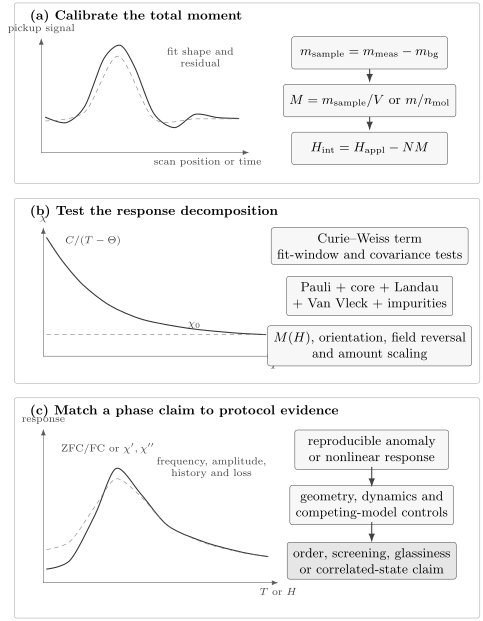
Magnetic-susceptibility inference proceeds from a calibrated total moment, through normalization, background and demagnetizing-field corrections, to a response decomposition and protocol-dependent phase tests. No single curve bypasses the middle stages.

Pauli Susceptibility

Noninteracting benchmark

An itinerant Fermi system responds because a magnetic field shifts the energies of opposite spin projections. Let $D^\ast(E_F)$ be the total quasiparticle density of states at the Fermi energy, including both spin species, per volume and energy. For an isotropic Zeeman coupling with effective $g$ factor,

$$\chi_{\mathrm{P}} = \mu_0 \frac{(g\mu_B)^2}{4} D^\ast(E_F).$$

For $g=2$, this becomes $\chi_{\mathrm P}=\mu_0\mu_B^2D^\ast(E_F)$. The formula is a benchmark, not a universal decomposition. Real materials can have anisotropic $g$ tensors, spin–orbit-entangled bands, multiple Fermi surfaces, exchange enhancement, and orbital response of comparable magnitude.

The electronic heat-capacity coefficient for the same quasiparticle density of states is

$$\gamma_V = \frac{\pi^2k_B^2}{3} D^\ast(E_F).$$

This motivates a generalized Wilson ratio

$$R_W = \frac{\pi^2k_B^2} {3\mu_0(g\mu_B/2)^2} \frac{\chi_{\mathrm{spin}}}{\gamma_V}.$$

The noninteracting benchmark is $R_W=1$ when the same degrees of freedom, normalization, and $g$ factor enter both quantities. Before quoting $R_W$, subtract non-spin terms from $\chi$, use either molar quantities for both numerator and denominator or volume quantities for both, and state the assumed $g$. An enhanced ratio can reflect ferromagnetic correlations, but uncertainty in orbital response or crystal-field anisotropy can imitate the enhancement.

What a flat susceptibility can mean

A weakly temperature-dependent positive susceptibility is compatible with Pauli paramagnetism, but it can also contain Van Vleck orbital mixing, core diamagnetism, and a broad exchange or coherence crossover. A useful fit model is

$$\chi(T) = \chi_{\mathrm{core}} + \chi_{\mathrm{Landau}} + \chi_{\mathrm{VV}} + \chi_{\mathrm{P}}(T) + \chi_{\mathrm{imp}}(T).$$

Calling the fitted constant $\chi_0$ “the Pauli susceptibility” silently assigns all temperature-independent terms to spin. Band calculations, anisotropy, NMR Knight shifts, and heat capacity can constrain that assignment. Stoner Criterion develops the exchange-enhanced spin response and its limits.

Curie and Curie–Weiss Regimes

Local moments

For independent, thermally randomized moments in the weak-field limit,

$$\chi_{\mathrm{mol}}(T) = \frac{C}{T}, \qquad C = \frac{\mu_0N_A\mu_{\mathrm{eff}}^2} {3k_B}.$$

Thus an SI molar Curie constant gives

$$\frac{\mu_{\mathrm{eff}}}{\mu_B} = \left( \frac{3k_BC} {\mu_0N_A\mu_B^2} \right)^{1/2}.$$

For an isolated angular-momentum multiplet with quantum number $J$ and Landé factor $g_J$,

$$\mu_{\mathrm{eff}} = g_J\sqrt{J(J+1)}\,\mu_B.$$

This effective moment is a high-temperature fluctuation scale, not the saturated moment $g_JJ\mu_B$. Confusing the two gives a systematic mismatch even for an ideal ion.

Interactions are often summarized by the Curie–Weiss form

$$\chi_{\mathrm{mol}}(T) = \chi_0 + \frac{C}{T-\Theta_{\mathrm{CW}}}.$$

Here $\Theta_{\mathrm{CW}}$ is a model-dependent intercept. In a simple local-moment mean-field model it reflects a weighted exchange scale, but its sign does not uniquely determine the eventual ordered state when interactions compete, sublattices are inequivalent, or anisotropic and long-range couplings matter.

Fit the regime, not the ruler

A straight-looking $1/\chi$ plot is not sufficient. If $\chi_0\neq0$, the linear quantity is

$$\frac{1}{\chi_{\mathrm{mol}}-\chi_0} = \frac{T-\Theta_{\mathrm{CW}}}{C},$$

and $\chi_0$, $C$, and $\Theta_{\mathrm{CW}}$ can be strongly covariant. Fit the untransformed $\chi(T)$ with uncertainties when possible, because inversion makes errors heteroscedastic and visually suppresses small systematic residuals.

The fit window should lie above the exchange, Kondo, ordering, and blocking scales while remaining within a temperature range where the same crystal-field manifold is active. A low-lying excited multiplet can curve $1/\chi$ without any change in exchange. Temperature-independent terms matter most at the high-temperature end, exactly where a broad fit may seem most convincing.

Useful robustness tests are:

• vary both lower and upper fit bounds and plot parameter drift;
• fit crystallographic directions separately before averaging;
• compare $C$ with the known magnetic-ion fraction and valence;
• inspect $M(H,T)$ for saturation, impurity tails, and nonlinearity;
• compare $\Theta_{\mathrm{CW}}$ with ordering, heat-capacity, and spectroscopic scales;
• report the full parameter covariance, not only marginal standard errors.

A large ratio $|\Theta_{\mathrm{CW}}|/T_{\mathrm{order}}$ is often called a frustration parameter. It is a useful screening metric only when the Curie–Weiss model is valid and $T_{\mathrm{order}}$ is independently established. Low dimensionality, anisotropy, disorder, Kondo screening, and a poor fit can also suppress or obscure ordering.

Diamagnetism and Orbital Response

Core, Landau, and Van Vleck terms

Closed electron shells generate core diamagnetism. Tabulated ionic increments can provide a rough subtraction, but covalency and solid-state charge distribution limit their accuracy. Conduction electrons also have orbital diamagnetism. For an ideal three-dimensional parabolic band with $g=2$,

$$\chi_{\mathrm{Landau}} = -\frac{1}{3}\chi_{\mathrm{P}}.$$

That ratio is not a general rule for multiband, low-dimensional, Dirac, flat-band, or strong spin–orbit systems. Near band degeneracies, orbital susceptibility can be large, anisotropic, and nonanalytic.

Virtual transitions between crystal-field or spin–orbit-coupled states generate Van Vleck susceptibility. In a simple nondegenerate single-ion picture, the molar response along direction $\alpha$ contains

$$\chi_{\mathrm{VV},\alpha}^{\mathrm{mol}} = 2\mu_0N_A \sum_{n\neq0} \frac{ \left| \langle n|\hat{\mu}_{\alpha}|0\rangle \right|^2 } {E_n-E_0}.$$

It is positive in this elementary form and can remain nearly temperature independent when the excited states are well above $k_BT$. Degeneracies, thermal populations, exchange, and band formation require a fuller treatment. Most importantly, a constant positive term need not come from a Fermi surface.

Superconducting screening

Diamagnetic onset is a powerful superconductivity diagnostic when its geometry and history are controlled. ZFC screening tests whether magnetic flux is excluded from much of the specimen after the field is applied at low temperature. Field-cooled magnetization probes flux expulsion under a different history and is often reduced by pinning. These are not interchangeable measurements.

A credible magnetic superconductivity claim states:

• field magnitude, direction, remanent-field procedure, and ZFC/FC sequence;
• raw moment, sample amount, density or dimensions, and demagnetizing correction;
• onset criterion and transition width;
• field dependence relative to lower critical and irreversibility scales;
• whether the signal scales with sample amount and survives holder controls;
• complementary zero resistance, heat capacity, local-field, microwave, or diffraction evidence as appropriate.

The ZFC shielding magnitude is not a direct superconducting volume fraction in a platelet, porous pellet, powder, granular composite, or specimen whose dimensions are comparable to the penetration depth. Conversely, a small field-cooled signal does not imply a small superconducting volume when vortex pinning is strong.

Ordered Phases

Ferromagnets

A ferromagnet is not identified merely by an upturn in $\chi(T)$. Bulk evidence includes a spontaneous equilibrium magnetization below the transition, anisotropy-consistent behavior, and reproducible field dependence after geometry correction. Real low-field measurements are dominated by domain nucleation, wall motion, pinning, and history. The measured susceptibility can therefore be very large, nonlinear, frequency dependent, and dissipative.

Record complete $M(H)$ loops with sweep rate and maximum-field history. Subtract holder and linear backgrounds without erasing the high-field approach to saturation. A small hysteretic component can come from a dilute ferromagnetic impurity even when the host is paramagnetic. Scaling of saturation moment with sample amount, composition, and impurity concentration is often decisive. Ferromagnetism owns spontaneous symmetry breaking, domains, Curie behavior near the transition, and Arrott analysis.

Antiferromagnets and ferrimagnets

The uniform susceptibility of an antiferromagnet commonly shows a cusp or slope change near the Néel temperature, but the shape depends strongly on anisotropy, dimensionality, domain population, and field direction. Short-range correlations can produce a broad maximum above the ordering temperature. The ordering wavevector is finite, so a uniform magnetometer does not directly measure the staggered order parameter.

For some simple antiferromagnets, Fisher’s relation motivates comparing the magnetic heat capacity with

$$\frac{d(\chi T)}{dT}.$$

This can sharpen a transition estimate, but it is not a universal identity for arbitrary anisotropic, itinerant, frustrated, or multi-sublattice magnets. Diffraction or a local magnetic probe is needed to establish the magnetic structure. Antiferromagnetism develops the staggered order parameter and its direct signatures.

Ferrimagnets contain oppositely aligned sublattices with unequal moments. Their inverse susceptibility can curve substantially, and a compensation temperature can drive the net moment through zero without destroying sublattice order. A one-component Curie–Weiss fit can therefore return parameters with little microscopic meaning. Ferrimagnetism owns the two-sublattice physics.

Glassiness, Blocking, and Slow Dynamics

A cusp in ac susceptibility that shifts with frequency, together with ZFC–FC splitting, signals slow magnetic dynamics. It does not by itself distinguish a collective spin glass from superparamagnetic blocking, domain-wall freezing, cluster glassiness, or vortex dynamics.

A compact empirical frequency-shift metric is

$$K = \frac{\Delta T_f} {T_f\,\Delta\log_{10}f},$$

where $T_f$ is a consistently defined peak or inflection temperature. Numerical ranges quoted for “canonical” spin glasses and superparamagnets overlap across materials and frequency windows, so $K$ is a comparator rather than a phase criterion.

For a noninteracting single-domain particle with anisotropy barrier $E_b=KV$, the simplest blocking model gives

$$\tau(T) = \tau_0 \exp\left( \frac{KV}{k_BT} \right).$$

The observed blocking temperature solves $\tau(T_B)\sim t_{\mathrm{obs}}$ and therefore depends on measurement time. A distribution of sizes produces broad peaks and relaxation. Interactions can make even this description inadequate.

A collective-glass claim should combine frequency and amplitude sweeps with aging, memory, nonlinear susceptibility, relaxation scaling, and a structural account of disorder. Local probes or scattering can test whether static moments develop throughout the sample. Glasses and Spin Glasses owns overlap order, aging, and the broader phase-theory evidence.

Spin-Liquid and Heavy-Fermion Signatures

Spin-liquid-compatible behavior

A frustrated magnet may show a Curie–Weiss regime at high temperature, broad susceptibility features as short-range correlations develop, and no sharp ordering anomaly down to the lowest measured temperature. Those observations are compatible with a quantum spin liquid, but they are also compatible with weak ordering below the base temperature, disorder, random singlets, glassiness, or a valence-bond state.

Low-temperature Curie tails are especially dangerous:

$$\chi(T) = \chi_{\mathrm{intrinsic}}(T) + \frac{C_{\mathrm{imp}}}{T-\Theta_{\mathrm{imp}}}.$$

A small fraction of orphan spins can dominate the bulk response while contributing little to the intrinsic correlations. Constrain that fraction with field dependence, saturation scale, composition, NMR line shapes, muon response, and diffuse scattering. Susceptibility can establish active moments, anisotropy, interaction scales, and absence of a bulk uniform anomaly within a stated window. It cannot by itself establish long-range entanglement or fractionalization. Quantum Spin Liquids owns the phase taxonomy and multimodal evidence standards.

Heavy-fermion-compatible behavior

Many $f$-electron materials cross from high-temperature local-moment Curie–Weiss behavior to a lower-temperature Kondo or lattice-coherence regime. The low-temperature susceptibility can become large and Pauli-like while the heat-capacity coefficient is also strongly enhanced. A broad maximum or anisotropic crossover may mark crystal-field depopulation, Kondo screening, intersite correlations, or coherence; susceptibility alone rarely separates them.

A disciplined heavy-fermion analysis:

• fits the local-moment regime above crystal-field, exchange, and coherence crossovers;
• compares $\mu_{\mathrm{eff}}$ with the expected ionic multiplet;
• reports anisotropy and field dependence;
• compares $\chi(T)$ with $C/T$, resistivity, Hall response, and spectroscopic coherence;
• forms a Wilson ratio only after subtracting core and orbital terms consistently;
• tests whether a low-temperature upturn scales as a dilute impurity contribution;
• distinguishes a crossover from a thermodynamic phase transition.

Heavy Fermions and Kondo Lattices own the microscopic and material-level interpretations. Quantum Criticality owns scaling and endpoint claims. Bulk susceptibility supplies one response channel in those arguments, not a verdict.

A Reproducible Analysis Workflow

Preserve the reduction chain

For each specimen and orientation, archive:

1. sample identifier, composition, mass, dimensions, mounting image, and field direction;
2. instrument mode, calibration state, scan or vibration parameters, and raw record;
3. holder, substrate, grease, and empty-probe controls;
4. magnet reset, remanent-field estimate, temperature and field history, sweep rates, and waiting times;
5. fitted moment with scan residuals or harmonic amplitudes;
6. amount normalization and SI conversion;
7. internal-field correction with geometry convention and uncertainty;
8. model, fit window, parameter covariance, residuals, and rejected alternatives;
9. replicate and orthogonal-probe checks supporting the final claim.

Keep raw moment, background-subtracted moment, $M$, $\chi_{\mathrm{app}}$, and corrected $\chi$ as separate data columns. Replacing one with the next destroys auditability.

Match claim to evidence

Claim	Minimum magnetic evidence	Essential controls or complements
Curie–Weiss local-moment regime	Stable $C$, $\Theta_{\mathrm{CW}}$, and $\chi_0$ over a justified window	Crystal-field scale, composition, anisotropy, fit covariance
Ferromagnetic component	Reproducible hysteretic or spontaneous component	Holder and contaminant scaling, demagnetization, microscopy or diffraction
Antiferromagnetic transition	Direction-resolved anomaly consistent across protocols	Heat capacity plus magnetic diffraction or local probe
Superconducting screening	Reproducible diamagnetic onset under stated ZFC/FC protocol	Geometry correction, zero resistance, bulk thermodynamic or local-field evidence
Spin glass	Frequency-dependent nonlinear freezing and irreversibility	Aging, memory, amplitude dependence, blocking alternatives
Heavy-fermion coherence	Enhanced low-temperature spin response correlated with other scales	$C/T$, transport, spectroscopy, crystal-field and impurity controls
Quantum-spin-liquid candidate	No order plus intrinsic correlated response over a declared window	Local probes, scattering continuum, thermodynamics, disorder controls

The table specifies floors, not sufficient conditions for every material. A surprising claim should require stronger controls, multiple specimens, and independent replication.

Common Mistakes

• Mixing $B$, $H_{\mathrm{appl}}$, and $H_{\mathrm{int}}$. State the derivative being reported and correct demagnetization where it matters.
• Dropping the SI–cgs factor. Molar cgs susceptibility converts with $4\pi\times10^{-6}$, not $10^{-6}$ alone.
• Calling $M/H$ a susceptibility in a hysteretic regime. Use differential response and preserve branch, rate, and history.
• Treating an instrument fit as raw truth. Inspect SQUID scan shape, VSM centering, and fit residuals.
• Subtracting a convenient high-field line. It may contain the intrinsic Pauli, Van Vleck, or unsaturated magnetic response.
• Fitting $1/\chi$ without $\chi_0$. The apparent intercept and moment can shift substantially.
• Equating $\mu_{\mathrm{eff}}$ with saturation moment. They involve $\sqrt{J(J+1)}$ and $J$, respectively.
• Reading the sign of $\Theta_{\mathrm{CW}}$ as the ordering pattern. Competing and multi-sublattice interactions defeat that shortcut.
• Calling ZFC–FC splitting a spin glass. Domains, particles, vortices, and structural hysteresis can do the same.
• Calling apparent shielding a volume fraction. Demagnetization, penetration depth, porosity, and granularity intervene.
• Calling a flat positive term Pauli susceptibility. Core, Landau, Van Vleck, and band-orbital terms must be assessed.
• Claiming a spin liquid or heavy fermion from $\chi(T)$ alone. Those are multimodal inferences.

Exercises

Exercise 1: Convert a molar susceptibility

A paper reports $\chi_{\mathrm{mol}}^{\mathrm{cgs}}=3.20\times10^{-3}\ \mathrm{cm^3\,mol^{-1}}$. Convert it to SI molar susceptibility.

Solution

Use the molar conversion including the $4\pi$ factor:

$$\begin{aligned} \chi_{\mathrm{mol}}^{\mathrm{SI}} &= 4\pi\times10^{-6} \left( 3.20\times10^{-3} \right) \ \mathrm{m^3\,mol^{-1}}\\ &= 4.02\times10^{-8} \ \mathrm{m^3\,mol^{-1}}. \end{aligned}$$

The numerical value is not $3.20\times10^{-9}$ because susceptibility conventions, not only cubic centimetres to cubic metres, contribute to the conversion.

Exercise 2: Correct a platelet’s apparent susceptibility

A platelet measured perpendicular to its face has $N=0.70$ and $\chi_{\mathrm{app}}=-2.50$. Find the internal-field susceptibility in the ellipsoidal approximation. Is the result compatible with nearly complete superconducting screening?

Solution

Apply

$$\chi = \frac{\chi_{\mathrm{app}}} {1-N\chi_{\mathrm{app}}}.$$

Therefore

$$\chi = \frac{-2.50} {1-(0.70)(-2.50)} = \frac{-2.50}{2.75} = -0.909.$$

The corrected value is close to the ideal SI value $-1$. The apparent magnitude larger than one is a geometry effect, not evidence for a superconducting fraction above $100\%$. A real platelet is not an ellipsoid, so uncertainty in the effective $N$ and finite penetration depth still matter.

Exercise 3: Extract an effective moment

An SI Curie–Weiss fit gives

$$C=1.26\times10^{-5}\ \mathrm{m^3\,K\,mol^{-1}}.$$

Find $\mu_{\mathrm{eff}}/\mu_B$. Compare it with a spin-only $S=1$ ion with $g=2$.

Solution

The Curie constant produced by one Bohr magneton squared is

$$\frac{\mu_0N_A\mu_B^2}{3k_B} \simeq 1.57\times10^{-6} \ \mathrm{m^3\,K\,mol^{-1}}.$$

Hence

$$\frac{\mu_{\mathrm{eff}}}{\mu_B} = \sqrt{ \frac{1.26\times10^{-5}} {1.57\times10^{-6}} } \simeq 2.83.$$

For $S=1$ and $g=2$,

$$g\sqrt{S(S+1)} = 2\sqrt{2} \simeq 2.83.$$

The Curie constant is therefore consistent with one such moment per formula unit, subject to occupancy, orbital, and fit-window checks. The corresponding saturation moment would be $gS\mu_B=2\mu_B$, not $2.83\mu_B$.

Exercise 4: Diagnose a neglected constant background

Suppose the true susceptibility is

$$\chi(T) = 3.0\times10^{-9} + \frac{1.26\times10^{-5}}{T+20} \quad \mathrm{m^3\,mol^{-1}}.$$

Using only the points at $100\ \mathrm K$ and $300\ \mathrm K$, estimate the apparent Curie–Weiss temperature obtained by forcing $1/\chi$ to be linear with no $\chi_0$ term.

Solution

At the two temperatures,

$$\begin{aligned} \chi(100\ \mathrm K) &= 1.08\times10^{-7} \ \mathrm{m^3\,mol^{-1}},\\ \chi(300\ \mathrm K) &= 4.2375\times10^{-8} \ \mathrm{m^3\,mol^{-1}}. \end{aligned}$$

Their inverses are approximately $9.26\times10^6$ and $2.36\times10^7\ \mathrm{mol\,m^{-3}}$. A line through these points has slope

$$a \simeq 7.17\times10^4 \ \mathrm{mol\,m^{-3}\,K^{-1}}$$

and intercept $b\simeq2.09\times10^6\ \mathrm{mol\,m^{-3}}$. Written as $a(T-\Theta_{\mathrm{app}})$, it gives

$$\Theta_{\mathrm{app}} = -\frac{b}{a} \simeq -29\ \mathrm K.$$

The true denominator contains $T+20$, so the true Curie–Weiss temperature is $-20\ \mathrm K$. Neglecting a small positive constant biases the inferred intercept by almost $50\%$ in this two-point example.

Exercise 5: AC loss

An ac experiment uses $h_{\mathrm{ac}}=80\ \mathrm{A\,m^{-1}}$ at $f=1.0\ \mathrm{kHz}$ and measures $\chi''=0.030$ under the convention defined above. Find the energy dissipated per unit volume per cycle and the average dissipated power density.

Solution

The loss per cycle is

$$\begin{aligned} W_{\mathrm{cycle}} &= \mu_0\pi h_{\mathrm{ac}}^2\chi''\\ &= \left( 4\pi\times10^{-7} \right) \pi(80)^2(0.030)\\ &\simeq 7.58\times10^{-4} \ \mathrm{J\,m^{-3}}. \end{aligned}$$

Multiplying by cycles per second,

$$\frac{P}{V} = fW_{\mathrm{cycle}} \simeq 0.758\ \mathrm{W\,m^{-3}}.$$

This is the sample’s magnetic loss density under the linear-response convention. Coil and eddy-current backgrounds still require independent subtraction.

Exercise 6: Wilson-ratio bookkeeping

Explain why it is invalid to combine a molar susceptibility that still contains core diamagnetism with a volumetric heat-capacity coefficient in a Wilson ratio. Give a valid workflow.

Solution

The ratio is dimensionless only when susceptibility and $\gamma$ refer to the same amount convention. Molar $\chi$ divided by volumetric $\gamma_V$ leaves an unphysical molar-volume factor. Core diamagnetism also does not arise from the low-energy quasiparticles counted by $\gamma$, so retaining it contaminates the spin response.

A valid workflow is:

1. convert both observables to molar quantities or both to volume quantities using a documented molar volume;
2. estimate and subtract core, Landau, Van Vleck, impurity, and ordered contributions to isolate $\chi_{\mathrm{spin}}$ as far as the data permit;
3. use the normal-state electronic $\gamma$ for the same specimen and regime;
4. state the effective $g$ factor and its direction;
5. propagate the subtraction and normalization uncertainties.

Only then can a deviation from the noninteracting value be interpreted as evidence for interaction-enhanced spin response.

Exercise 7: Audit a spin-liquid claim

A frustrated insulator has $\Theta_{\mathrm{CW}}=-120\ \mathrm K$, no sharp anomaly in $\chi(T)$ above $2\ \mathrm K$, and a low-temperature Curie tail. The authors call it a quantum spin liquid. What can the susceptibility establish, and what measurements are needed before the phase claim is credible?

Solution

The data can establish a high-temperature antiferromagnetic interaction scale if the Curie–Weiss window and crystal-field assumptions are valid. They can also establish the absence of a resolved bulk uniform-susceptibility anomaly above $2\ \mathrm K$. They do not distinguish a quantum spin liquid from ordering below $2\ \mathrm K$, weak or broadened order, a spin glass, random singlets, a valence-bond state, or disorder.

The Curie tail should first be tested against a dilute-moment model using field dependence and saturation, chemical analysis, and local line shapes. Heat capacity should test for bulk anomalies and entropy release. Muon or nuclear-resonance measurements should test for static internal fields and heterogeneous freezing. Neutron scattering should search for magnetic Bragg peaks and characterize diffuse or continuum response. AC susceptibility, aging, and memory should test glassiness. Measurements should extend below the lowest inferred intrinsic scale and be repeated across specimens.

A defensible intermediate statement is “a frustrated magnet with no detected long-range order above $2\ \mathrm K$ and a low-temperature response requiring impurity or intrinsic modeling.” Quantum spin liquid remains a hypothesis until orthogonal evidence excludes the principal alternatives.

Research Status

• Established: SI field and susceptibility relations; SQUID and VSM transduction; Curie, Pauli, Landau, and Van Vleck benchmarks in their stated regimes; ellipsoidal demagnetizing fields; ac response and loss; bulk signatures of conventional magnetic order and superconducting screening.
• Model dependent: background decomposition, effective demagnetizing factors for nonellipsoids, Curie–Weiss windows, ionic moment assignments, Pauli and orbital separation, Wilson ratios, superconducting shielding fractions, and relaxation fits.
• Active: orbital susceptibility in topological and flat-band systems; disentangling Kondo, crystal-field, and quantum-critical crossovers; disorder-aware inference in frustrated magnets; quantitative multimodal fusion of magnetometry, calorimetry, scattering, and local probes.
• Unsupported when used alone: declaring a spin liquid from absent order, a spin glass from one frequency-shifting cusp, heavy-fermion coherence from a large $\chi$, or a superconducting volume fraction from uncorrected ZFC shielding.

Connections

• Magnetic Moments in Matter compares the Curie-effective moment inferred here with saturation, ordered, and fluctuating moments only after their state, normalization, and probe windows are aligned.
• How Quantum Matter Is Measured supplies the general record-to-observable-to-claim framework.
• Vortex Matter, Pinning, and Flux Flow interprets irreversible magnetization, ac loss, relaxation, and field-history dependence as barriers, pinning, creep, or collective vortex response after the magnetometry and demagnetization corrections owned here.
• Data Interpretation and Pitfalls compares equilibrium hysteresis, finite-rate lag, sample variation, phase mixtures, and cross-probe evidence.
• Heat Capacity and Thermodynamics tests bulk transitions, entropy release, Sommerfeld coefficients, and magnetic Schottky backgrounds.
• Neutron Scattering measures magnetic ordering wavevectors, moments, spin waves, diffuse correlations, and continua.
• Susceptibilities develops static, dynamic, uniform, finite-wavevector, tensor, and source conventions.
• Fluctuations and Susceptibilities derives equilibrium fluctuation-response identities.
• Stoner Criterion derives exchange enhancement and the uniform itinerant instability.
• Ferromagnetism, Antiferromagnetism, and Ferrimagnetism own the phase theories and direct order diagnostics.
• Magnetic Anisotropy develops crystal, shape, surface, and exchange anisotropies.
• Glasses and Spin Glasses develops collective freezing, overlap order, aging, and memory.
• Heavy Fermions and Kondo Lattices place susceptibility crossovers in a multimodal coherence problem.
• Quantum Spin Liquids develops the evidence needed beyond absence of order.
• Magnetometry develops quantum sensors that measure magnetic fields rather than bulk material response.

References

1. J. H. Van Vleck, The Theory of Electric and Magnetic Susceptibilities (Oxford University Press, 1932). The foundational quantum treatment of atomic, molecular, and solid-state susceptibility.
2. S. Foner, “Versatile and Sensitive Vibrating-Sample Magnetometer,” Review of Scientific Instruments 30, 548–557 (1959), doi:10.1063/1.1716679.
3. J. Clarke and A. I. Braginski, eds., The SQUID Handbook, Volume I: Fundamentals and Technology of SQUIDs and SQUID Systems (Wiley-VCH, 2004), doi:10.1002/3527603646.
4. J. A. Osborn, “Demagnetizing Factors of the General Ellipsoid,” Physical Review 67, 351–357 (1945), doi:10.1103/PhysRev.67.351.
5. A. Aharoni, “Demagnetizing Factors for Rectangular Ferromagnetic Prisms,” Journal of Applied Physics 83, 3432–3434 (1998), doi:10.1063/1.367113.
6. R. Prozorov and V. G. Kogan, “Effective Demagnetizing Factors of Diamagnetic Samples of Various Shapes,” Physical Review Applied 10, 014030 (2018), doi:10.1103/PhysRevApplied.10.014030.
7. S. Blundell, Magnetism in Condensed Matter (Oxford University Press, 2001), doi:10.1093/oso/9780198505921.001.0001.
8. B. D. Cullity and C. D. Graham, Introduction to Magnetic Materials, 2nd ed. (Wiley, 2008), doi:10.1002/9780470386323.
9. A. H. Morrish, The Physical Principles of Magnetism (Wiley, 1965). A detailed reference on magnetic units, domains, anisotropy, and measurement.
10. E. C. Stoner, “Collective Electron Ferromagnetism,” Proceedings of the Royal Society A 165, 372–414 (1938), doi:10.1098/rspa.1938.0066.
11. K. G. Wilson, “The Renormalization Group: Critical Phenomena and the Kondo Problem,” Reviews of Modern Physics 47, 773–840 (1975), doi:10.1103/RevModPhys.47.773.
12. D. C. Johnston, “Magnetic Susceptibility of Collinear and Noncollinear Heisenberg Antiferromagnets,” Physical Review Letters 109, 077201 (2012), doi:10.1103/PhysRevLett.109.077201.
13. M. E. Fisher, “Relation Between the Specific Heat and Susceptibility of an Antiferromagnet,” Philosophical Magazine 7, 1731–1743 (1962), doi:10.1080/14786436208213705.
14. J. A. Mydosh, Spin Glasses: An Experimental Introduction (Taylor & Francis, 1993), doi:10.1201/9781482295191.
15. C. P. Bean and J. D. Livingston, “Superparamagnetism,” Journal of Applied Physics 30, S120–S129 (1959), doi:10.1063/1.2185850.
16. M. Tinkham, Introduction to Superconductivity, 2nd ed. (McGraw-Hill, 1996). Develops Meissner screening, critical fields, vortices, and geometry-dependent magnetic response.
17. L. Balents, “Spin Liquids in Frustrated Magnets,” Nature 464, 199–208 (2010), doi:10.1038/nature08917.
18. G. R. Stewart, “Heavy-Fermion Systems,” Reviews of Modern Physics 56, 755–787 (1984), doi:10.1103/RevModPhys.56.755.
19. A. P. Ramirez, “Strongly Geometrically Frustrated Magnets,” Annual Review of Materials Science 24, 453–480 (1994), doi:10.1146/annurev.ms.24.080194.002321.
20. Joint Committee for Guides in Metrology, Evaluation of Measurement Data—Guide to the Expression of Uncertainty in Measurement, JCGM 100:2008 (2008), doi:10.59161/JCGM100-2008E.

Summary

Magnetic susceptibility becomes physically meaningful only after the measured moment has been centered, background-subtracted, normalized, assigned a field convention, and corrected for geometry where necessary. Pauli, Curie–Weiss, core, Landau, Van Vleck, ordered, superconducting, impurity, and dynamical responses can overlap in the same curve. Field sweeps, reversal, orientation, ZFC/FC history, frequency and amplitude dependence, fit-window stability, and orthogonal probes separate those possibilities. The strongest conclusion is the highest rung supported by that complete evidence chain, not the most dramatic label compatible with one feature.