Fluctuations and Susceptibilities

Equilibrium fluctuations and static susceptibilities are two descriptions of how weakly constrained a macroscopic quantity is. A broad equilibrium distribution means that nearby values cost little thermodynamic weight; a source conjugate to that quantity can then shift its mean strongly. For a canonical state with a linear source,

$$H_f = H_0-fB,$$

the isothermal response of an observable $A$ is

$$\chi_T^{AB} = \left. \frac{\partial\langle A\rangle_f} {\partial f} \right|_{f=0}.$$

If $A$ has no explicit source dependence, the exact quantum identity is

$$\chi_T^{AB} = \beta\, \operatorname{Cov}_{\mathrm{KM}}(A,B),$$

where $\operatorname{Cov}_{\mathrm{KM}}$ is the Kubo–Mori covariance. The familiar formula

$$\chi_T^{BB} = \beta\operatorname{Var}(B)$$

is recovered when $B$ commutes with the equilibrium density operator, in particular when $[B,H_0]=0$. Replacing the Kubo–Mori covariance by an ordinary equal-time variance without checking this condition is one of the most important quantum corrections to classical fluctuation intuition.

Three standard special cases are

$$\operatorname{Var}(E) = k_{\mathrm B}T^2C_V,$$ $$\operatorname{Var}(N) = k_{\mathrm B}T,Vn^2\kappa_T,$$

and, for a commuting magnetization $M$ coupled through $-BM$,

$$\frac{1}{V} \left( \frac{\partial\langle M\rangle} {\partial B} \right)_T = \frac{\beta}{V} \operatorname{Var}(M).$$

Each formula silently specifies an ensemble, held-fixed variables, source convention, normalization, and equilibration protocol. This page develops those qualifications rather than treating fluctuation formulas as context-free substitutions.

Canonical Scope

This page is the canonical home for:

• equilibrium fluctuations as variances and covariances;
• static isothermal response from source-dependent equilibrium states;
• the Kubo–Mori replacement required by noncommuting observables;
• energy–heat-capacity, number–compressibility, and magnetization–susceptibility identities;
• covariance matrices, cross responses, and stability;
• ensemble dependence, thermodynamic scaling, and critical enhancement;
• practical diagnostics for applying fluctuation formulas.

Partition Functions owns the thermodynamic source-generating machinery. Connected Correlation Functions owns the operator cumulant hierarchy, clustering, and extensive-sum scaling. Thermodynamic Potentials owns Legendre transforms, natural variables, and the complete curvature dictionary. Maximum Entropy Principle owns the Kubo–Mori Hessian as the information geometry of an exponential family.

Real-time response is a different layer. Kubo Formula owns retarded commutators, contact terms, conductivity, and orders of static and uniform limits. Fluctuation–Dissipation Theorem owns the general frequency-dependent KMS relation between many-body fluctuations and dissipative response. Sum Rules owns positive and inverse spectral moments and explains when a zero-frequency retarded limit differs from a re-equilibrated thermodynamic derivative. Fluctuation–Dissipation Relation owns bath-noise and damping applications. The present page concerns re-equilibrated static states unless stated otherwise.

What Counts as a Fluctuation?

For a Hermitian observable $A$ in a state $\rho$, define

$$\Delta A = A-\langle A\rangle_\rho\mathbb I,$$ $$\operatorname{Var}_\rho(A) = \langle(\Delta A)^2\rangle_\rho,$$

and

$$\operatorname{Cov}_\rho(A,B) = \frac{1}{2} \langle \Delta A\Delta B + \Delta B\Delta A \rangle_\rho.$$

The symmetrized covariance is real for Hermitian $A$ and $B$. When the observables commute, it reduces to the ordinary classical covariance of their joint outcome distribution.

The word fluctuation is used for several related but distinct objects:

1. Outcome fluctuation: the spread of repeated projective measurements of $A$ in the fixed state $\rho$.
2. Ensemble fluctuation: the spread of quantities such as energy or particle number across the sectors weighted by an equilibrium ensemble.
3. Temporal noise: the time-dependent random signal or correlation spectrum produced by a detector coupled to the system.

The first is always defined by the quantum variance. The second becomes an ordinary distribution over sectors when the fluctuating quantity commutes with the equilibrium state. The third depends on dynamics, operator ordering, detector conventions, and bandwidth. It cannot generally be reconstructed from one equal-time variance.

There is also no decomposition-independent split of a mixed-state variance into “classical ignorance” and “quantum uncertainty.” A density operator has many pure-state decompositions. If a particular preparation ensemble is operationally specified, a law-of-total-variance decomposition may be useful, but it belongs to that preparation, not to $\rho$ alone.

Ensemble Dependence

Whether a global quantity fluctuates is part of the ensemble definition.

Ensemble	Controlled variables	Global quantities fixed by construction	Typical global fluctuations
microcanonical	$E,V,N$	energy shell and particle sector	observables within the shell
canonical	$T,V,N$	particle number	energy and unconstrained observables
grand canonical	$T,V,\mu$	neither $E$ nor $N$	energy, particle number, and their covariance

An idealized microcanonical state has zero variance of the coarse-grained shell label, while a canonical state has nonzero energy variance. A canonical fixed-$N$ state has

$$\operatorname{Var}(N)=0,$$

whereas a grand-canonical state generally does not. These statements do not imply that the corresponding material has zero heat capacity or compressibility. A response coefficient compares nearby equilibrium states as a control variable changes; a global variance describes the distribution inside one specified ensemble.

For ordinary short-range systems, local observables can agree across ensembles in the thermodynamic limit even when global fluctuations remain different. Ensemble Equivalence explains the conditions and failures of that statement.

Source-Dependent Equilibrium States

Let

$$H_f = H_0-fB$$

with $B=B^\dagger$, and define

$$Z_f = \operatorname{Tr}e^{-\beta H_f}, \qquad \rho_f = \frac{e^{-\beta H_f}}{Z_f}.$$

The sign convention matters: positive $f$ energetically favors larger $B$. The first derivative of the free energy

$$F(f) = -\frac{1}{\beta}\ln Z_f$$

is

$$\frac{\partial F}{\partial f} = -\langle B\rangle_f.$$

This identity is exact even if $B$ does not commute with $H_f$. It follows from the Duhamel derivative

$$\frac{\partial e^{-\beta H_f}} {\partial f} = \beta \int_0^1ds\, e^{-(1-s)\beta H_f} B e^{-s\beta H_f}$$

and cyclicity of the trace.

The second derivative probes response:

$$-\frac{\partial^2F}{\partial f^2} = \frac{\partial\langle B\rangle_f} {\partial f} = \chi_T^{BB}(f).$$

Thus a free energy is concave in a linearly coupled field. The susceptibility is nonnegative for a stable diagonal source–detector pair under these conventions.

The Kubo–Mori Covariance

For a full-rank equilibrium state $\rho$, define

$$\operatorname{Cov}_{\mathrm{KM},\rho}(A,B) = \int_0^1ds\, \operatorname{Tr} \left( \rho^s\Delta A\, \rho^{1-s}\Delta B \right).$$

The definition extends to rank-deficient states by a suitable limit on the support when that limit exists. For Hermitian observables it is symmetric, and

$$\operatorname{Cov}_{\mathrm{KM}}(A,A) \geq 0.$$

In an eigenbasis of $\rho$,

$$\rho = \sum_n p_n \lvert n\rangle\langle n\rvert,$$

one obtains

$$\operatorname{Cov}_{\mathrm{KM}}(A,A) = \sum_{n,m} L(p_n,p_m) \left| \langle n\lvert\Delta A\rvert m\rangle \right|^2,$$

where the logarithmic mean is

$$L(x,y) = \begin{cases} \dfrac{x-y}{\ln x-\ln y},&x\neq y,\\ x,&x=y. \end{cases}$$

Every coefficient is nonnegative. If $[A,\rho]=0$, only matrix elements inside equal-$p$ blocks survive and

$$\operatorname{Cov}_{\mathrm{KM}}(A,A) = \operatorname{Var}(A).$$

For $\rho=e^{-\beta H}/Z$, the same object has the imaginary-time form

$$\beta\operatorname{Cov}_{\mathrm{KM}}(A,B) = \int_0^\beta d\lambda\, \left\langle \Delta A(-i\hbar\lambda) \Delta B(0) \right\rangle,$$

with

$$A(-i\hbar\lambda) = e^{\lambda H}Ae^{-\lambda H}.$$

The isothermal source response is therefore

$$\chi_T^{AB} = \beta\operatorname{Cov}_{\mathrm{KM}}(A,B)$$

when $A$ has no explicit $f$ dependence. The imaginary-time integral, not an arbitrary equal-time ordering, is the generally correct quantum static correlator.

Explicit Source Dependence

Suppose the Hamiltonian is a nonlinear function $H(f)$ and define the generalized displacement

$$B_f = -\frac{\partial H(f)}{\partial f}.$$

Then

$$\frac{\partial F}{\partial f} = -\langle B_f\rangle_f$$

and

$$\frac{\partial\langle B_f\rangle_f} {\partial f} = \left\langle \frac{\partial B_f}{\partial f} \right\rangle_f + \beta \operatorname{Cov}_{\mathrm{KM},f}(B_f,B_f).$$

The first term is an explicit-source or contact contribution. For a strictly linear coupling, $B_f=B$ and it vanishes. For electromagnetic response, elastic coordinates, and source-dependent effective operators, omitting it can give the wrong static limit.

The same structure holds for a detector $A(f)$ distinct from the coupled operator:

$$\frac{\partial\langle A(f)\rangle_f} {\partial f} = \left\langle \frac{\partial A}{\partial f} \right\rangle_f + \beta \operatorname{Cov}_{\mathrm{KM},f}(A,B_f).$$

Classical Tilting Intuition

When $X$ commutes with the equilibrium state, the source simply tilts its probability distribution:

$$P_f(X) = \frac{ P_0(X)e^{\beta fX} }{ \left\langle e^{\beta fX}\right\rangle_0 }.$$

Differentiating at $f=0$ gives

$$\left. \frac{\partial\langle X\rangle_f} {\partial f} \right|_{f=0} = \beta\operatorname{Var}_0(X).$$

For a Gaussian distribution,

$$P_0(X) \propto \exp \left[ -\frac{(X-\overline X)^2}{2\sigma_X^2} \right],$$

the tilted mean is

$$\langle X\rangle_f = \overline X + \beta\sigma_X^2f.$$

A broader distribution therefore produces a steeper linear response.

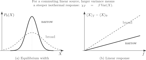
For a commuting observable with a linear conjugate source, equilibrium width and isothermal response carry the same information. The broad distribution has the larger variance and therefore the larger slope $\chi_T=\beta\operatorname{Var}(X)$. Noncommuting quantum observables require the Kubo–Mori covariance instead.

This picture is local. Far from $f=0$, higher cumulants control nonlinear response. Near phase coexistence, $P_0(X)$ can be bimodal rather than Gaussian, and one variance no longer describes its shape.

Energy Fluctuations and Heat Capacity

In the canonical ensemble,

$$\rho_\beta = \frac{e^{-\beta H}}{Z}, \qquad Z = \operatorname{Tr}e^{-\beta H},$$

with a temperature-independent Hamiltonian. Because $H$ commutes with $\rho_\beta$,

$$U = \langle H\rangle = -\frac{\partial\ln Z}{\partial\beta}$$

and

$$\frac{\partial U}{\partial\beta} = -\operatorname{Var}(H).$$

Using

$$\frac{d\beta}{dT} = -\frac{1}{k_{\mathrm B}T^2},$$

the constant-volume heat capacity is

$$\begin{aligned} C_V &= \left( \frac{\partial U}{\partial T} \right)_{V,N} \\ &= k_{\mathrm B}\beta^2 \operatorname{Var}(H). \end{aligned}$$

Equivalently,

$$\operatorname{Var}(E) = k_{\mathrm B}T^2C_V.$$

This is exact for the canonical ensemble under the assumptions above. It immediately gives

$$C_V\geq0$$

for a finite temperature-independent Hamiltonian with a convergent partition function. It does not prove nonnegative heat capacity in every ensemble. Microcanonical long-range and nonadditive systems require separate stability analysis.

If $C_V=c_VV$ is extensive, then

$$\operatorname{Var}(E) = k_{\mathrm B}T^2c_VV,$$

so the standard deviation grows as $V^{1/2}$ while a nonzero bulk mean energy grows as $V$. Relative fluctuations then scale as $V^{-1/2}$. The statement should not be expressed as $\Delta E/U$ when the chosen zero makes $U$ vanish or changes sign; the scaling of the intensive energy $e=E/V$ is unambiguous:

$$\operatorname{Var}(e) = \frac{k_{\mathrm B}T^2c_V}{V}.$$

The Canonical Ensemble develops the full energy distribution, Schottky anomaly, and oscillator examples. Here the formula serves as one member of a unified response dictionary.

Number Fluctuations and Compressibility

For a grand-canonical state,

$$\rho_{\mathrm G} = \frac{ e^{-\beta(H-\mu N)} }{\Xi},$$

ordinary equilibrium requires the charge to be conserved,

$$[H,N]=0.$$

Then

$$\overline N = \frac{1}{\beta} \frac{\partial\ln\Xi}{\partial\mu}$$

and

$$\left( \frac{\partial\overline N}{\partial\mu} \right)_{T,V} = \beta\operatorname{Var}(N).$$

For a homogeneous one-component system with density

$$n = \frac{\overline N}{V},$$

the isothermal compressibility is

$$\kappa_T = \frac{1}{n^2} \left( \frac{\partial n}{\partial\mu} \right)_T.$$

Therefore

$$\kappa_T = \frac{ \beta\operatorname{Var}(N) }{ Vn^2 }$$

or

$$\operatorname{Var}(N) = k_{\mathrm B}T\,Vn^2\kappa_T.$$

This relation is sometimes called the compressibility sum rule. It requires consistent definitions: some authors call

$$\kappa_n = \left( \frac{\partial n}{\partial\mu} \right)_T$$

the density susceptibility, while $\kappa_T=\kappa_n/n^2$ is the thermodynamic compressibility. The factors of $V$, $n$, and $n^2$ are not optional conventions.

Why fixed particle number is not zero compressibility

In a canonical ensemble,

$$\operatorname{Var}_{N}(N)=0$$

by construction. A finite compressibility can still be obtained from the curvature of the fixed-$N$ Helmholtz free energy, from the equation of state, or from an appropriate long-wavelength density response. The grand-canonical global-variance formula and the canonical free-energy derivative are alternative equilibrium representations under conditions of ensemble equivalence; they are not identities inside the same finite ensemble.

At exactly zero wavevector, the density operator is total $N$. If $N$ is conserved, its isolated finite-frequency retarded self-response vanishes. The thermodynamic derivative instead compares re-equilibrated states with different $\mu$. This is an order-of-limits issue, not a contradiction.

Strict zero temperature

For a finite system at $T=0$, the grand-canonical ground state usually lies in one definite-$N$ sector except at a level crossing. Then $\operatorname{Var}(N)=0$ and $\overline N(\mu)$ is stepwise constant. A smooth finite compressibility emerges only after an appropriate thermodynamic and zero-temperature limit. The expression $\beta\operatorname{Var}(N)$ must therefore be interpreted as a limit, not as the product of two separately evaluated quantities $\infty$ and $0$.

Magnetization Fluctuations and Susceptibility

For one field component, choose

$$H(B) = H_0-BM.$$

The total isothermal susceptibility is

$$\chi_{M,T} = \left( \frac{\partial\langle M\rangle} {\partial B} \right)_T.$$

If $[M,H_0]=0$, then

$$\chi_{M,T} = \beta\operatorname{Var}(M).$$

For a bulk susceptibility, define

$$\chi_T = \frac{1}{V}\chi_{M,T} = \frac{\beta}{V} \operatorname{Var}(M).$$

Depending on electromagnetic unit conventions, additional factors such as $\mu_0$ may be included in the definition of susceptibility or field. The Hamiltonian coupling determines the convention safely.

Independent moments and the Curie law

Consider $N_s$ independent two-state magnetic moments $m s_i$, with $s_i=\pm1$:

$$M = m\sum_{i=1}^{N_s}s_i, \qquad H(B) = -BM.$$

The one-site partition function is

$$Z_1 = 2\cosh(\beta mB),$$

and

$$\langle M\rangle = N_sm\tanh(\beta mB).$$

Thus

$$\chi_{M,T} = N_s\beta m^2 \operatorname{sech}^2(\beta mB).$$

The independent-site variance is

$$\operatorname{Var}(M) = N_sm^2 \operatorname{sech}^2(\beta mB),$$

which verifies $\chi_{M,T}=\beta\operatorname{Var}(M)$. At zero field,

$$\chi_T = \frac{n_sm^2}{k_{\mathrm B}T},$$

where $n_s=N_s/V$. This is the Curie law for independent moments.

Interactions can enhance, suppress, or singularly reorganize these fluctuations. A Curie–Weiss fit is not by itself evidence for independent spins, and a susceptibility peak in a finite sample is not by itself proof of a phase transition.

The Kondo Model Preview gives a canonical impurity example: a high-temperature Curie moment crosses over to a finite low-temperature susceptibility when an antiferromagnetic conduction bath screens the spin.

The Noncommuting Quantum Correction

The ordinary variance formula can fail dramatically when the source-coupled observable does not commute with the unperturbed Hamiltonian.

Consider a harmonic oscillator under a static force:

$$H_f = \frac{p^2}{2m} + \frac{1}{2}m\omega^2x^2 - fx.$$

Completing the square gives

$$H_f = \frac{p^2}{2m} + \frac{1}{2}m\omega^2 \left( x- \frac{f}{m\omega^2} \right)^2 - \frac{f^2}{2m\omega^2}.$$

Therefore

$$\langle x\rangle_f = \frac{f}{m\omega^2}, \qquad \chi_T^{xx} = \frac{1}{m\omega^2}.$$

At $f=0$, however,

$$\operatorname{Var}(x) = \frac{\hbar}{2m\omega} \coth \left( \frac{\beta\hbar\omega}{2} \right).$$

Hence

$$\beta\operatorname{Var}(x) = \frac{\beta\hbar}{2m\omega} \coth \left( \frac{\beta\hbar\omega}{2} \right)$$

is not $1/(m\omega^2)$ except in the high-temperature limit. At low temperature it even grows proportional to $\beta$ because the equal-time variance retains zero-point fluctuations.

The Kubo–Mori expression gives the correct answer. With

$$\overline n = \frac{1}{e^{\beta\hbar\omega}-1},$$

the imaginary-time correlator is

$$\begin{aligned} \langle x(-i\hbar\lambda)x(0)\rangle = \frac{\hbar}{2m\omega} \bigl[ &(\overline n+1)e^{-\lambda\hbar\omega} \\ &+ \overline n e^{\lambda\hbar\omega} \bigr]. \end{aligned}$$

Integrating gives

$$\int_0^\beta d\lambda\, \langle x(-i\hbar\lambda)x(0)\rangle = \frac{1}{m\omega^2}.$$

The static displacement susceptibility is controlled by the imaginary-time average. Equal-time zero-point uncertainty is physically real, but it is not interchangeable with a re-equilibrated force response.

Several Sources and Cross Susceptibilities

For linear sources

$$H(\mathbf f) = H_0- \sum_b f_bB_b,$$

define

$$\chi_{ab} = \frac{\partial\langle B_a\rangle} {\partial f_b}.$$

The equilibrium response matrix is

$$\chi_{ab} = \beta \operatorname{Cov}_{\mathrm{KM}}(B_a,B_b).$$

For real fields and Hermitian observables,

$$\chi_{ab} = \chi_{ba},$$

provided both derivatives refer to the same equilibrium potential and held-fixed variables. This is a static Maxwell reciprocity relation, not a generic statement about nonequilibrium retarded cross response.

For any real coefficients $c_a$, let

$$C = \sum_a c_aB_a.$$

Then

$$\sum_{a,b}c_a\chi_{ab}c_b = \beta \operatorname{Cov}_{\mathrm{KM}}(C,C) \geq 0.$$

The susceptibility matrix is therefore positive semidefinite. A zero eigenvalue can signal a redundant source direction, an exact constraint, or an operator combination that is constant on the support of the state.

When all relevant observables commute, positivity yields the covariance inequality

$$\operatorname{Cov}(A,B)^2 \leq \operatorname{Var}(A) \operatorname{Var}(B).$$

This inequality bounds cross responses by diagonal susceptibilities.

Energy–Number Cross Fluctuations

In grand-canonical equilibrium with $[H,N]=0$,

$$\Xi = \operatorname{Tr} e^{-\beta(H-\mu N)}.$$

At fixed $T$,

$$\left( \frac{\partial U}{\partial\mu} \right)_{T,V} = \beta\operatorname{Cov}(H,N).$$

At fixed $\mu$,

$$\left( \frac{\partial\overline N}{\partial\beta} \right)_{\mu,V} = -\operatorname{Cov} \left( N,H-\mu N \right).$$

The grand-Hamiltonian variance is

$$\begin{aligned} \operatorname{Var}(H-\mu N) = {}&\operatorname{Var}(H) + \mu^2\operatorname{Var}(N) \\ &- 2\mu\operatorname{Cov}(H,N). \end{aligned}$$

Consequently, a temperature derivative at fixed $\mu$ does not isolate $\operatorname{Var}(H)$. The derivative path through thermodynamic parameter space must be stated.

Local Correlations and Bulk Response

Let an extensive observable be a sum of local densities,

$$X = \sum_i x_i.$$

For commuting equal-time variables,

$$\operatorname{Var}(X) = \sum_{i,j} \langle\Delta x_i\Delta x_j\rangle.$$

In a homogeneous continuum system,

$$\frac{\operatorname{Var}(X)}{V} = \int d^dr\, C_{xx}(\mathbf r),$$

where

$$C_{xx}(\mathbf r) = \langle \Delta x(\mathbf r) \Delta x(\mathbf 0) \rangle.$$

Thus a bulk commuting susceptibility per volume obeys

$$\frac{\chi_T^{XX}}{V} = \beta \int d^dr\, C_{xx}(\mathbf r).$$

This identity explains why long-ranged correlations enhance susceptibilities. If $C_{xx}$ decays rapidly enough, the spatial integral is finite and $\operatorname{Var}(X)\sim V$. If a correlation length diverges or correlations decay too slowly, the integral can grow with system size.

For particle density,

$$\operatorname{Var}(N) = \int_Vd^dr \int_Vd^dr'\, \langle \Delta n(\mathbf r) \Delta n(\mathbf r') \rangle.$$

With the common static-structure-factor normalization

$$S(\mathbf 0) = \frac{\operatorname{Var}(N)}{\overline N},$$

the finite-temperature grand-canonical compressibility relation becomes

$$S(\mathbf 0) = n k_{\mathrm B}T\kappa_T.$$

Finite windows, exact global conservation, boundaries, and nonuniform density modify the naive $\mathbf q=0$ identification. Correlation Functions Overview develops connected correlators and spatial ordering conventions.

Thermodynamic-Limit Scaling

Away from criticality, an additive system with finite correlation length typically has

$$\langle X\rangle \sim V, \qquad \operatorname{Var}(X) \sim V.$$

Therefore

$$\Delta X \sim V^{1/2}$$

and, when the mean density is nonzero,

$$\frac{\Delta X}{|\langle X\rangle|} \sim V^{-1/2}.$$

Macroscopic relative fluctuations vanish even though the absolute fluctuation grows. This concentration is one reason deterministic thermodynamics emerges from statistical mechanics.

For the intensive variable $x=X/V$,

$$\operatorname{Var}(x) \sim V^{-1}.$$

If its distribution has a large-deviation form

$$P(x) \asymp e^{-\beta Vg(x)},$$

and $g$ has a regular minimum at $x_\star$, then

$$g(x) \simeq g(x_\star) + \frac{1}{2}g''(x_\star) (x-x_\star)^2.$$

The Gaussian width and response per volume are

$$\operatorname{Var}(x) \simeq \frac{1}{\beta Vg''(x_\star)},$$ $$\frac{1}{V} \frac{\partial\langle X\rangle}{\partial f} \simeq \frac{1}{g''(x_\star)}.$$

Small curvature means both broad fluctuations and large response.

Criticality and Phase Coexistence

A susceptibility can diverge only after an appropriate thermodynamic limit. For every finite system with a finite-dimensional Hilbert space, the partition function is analytic at finite temperature and source, and equilibrium susceptibilities are finite. Numerical or experimental finite systems display rounded peaks.

Near a continuous transition, a growing correlation length can make

$$\int d^dr\,C_{xx}(\mathbf r)$$

diverge. Then $\operatorname{Var}(X)$ grows faster than $V$, ordinary central-limit scaling fails, and the susceptibility acquires finite-size scaling governed by critical exponents.

At first-order coexistence, the order-parameter distribution may be bimodal. If the two peaks differ by an extensive amount of order $V$, then the between-peak contribution can scale as

$$\operatorname{Var}(X) \sim V^2.$$

The susceptibility per volume can then grow as $V$ at coexistence. This is phase switching, not a single broad Gaussian phase.

Finite-Temperature Phase Transitions owns the thermal-transition classification, critical-temperature conventions, finite-size rounding, and two-phase scaling that give these fluctuation signatures their interpretation.

Long-range interactions, nonadditive systems, constraints, and disorder can alter these scaling statements. The Thermodynamic Limit page states the order of limits and additivity assumptions in detail.

Static Thermodynamic Versus Retarded Response

The isothermal susceptibility compares equilibrium states:

$$\chi_T^{BB} = \left. \frac{\partial\langle B\rangle_f} {\partial f} \right|_{f=0}.$$

The retarded susceptibility instead asks how an isolated or weakly open system evolves after a time-dependent perturbation:

$$\chi_{BB}^R(t) = \frac{i}{\hbar} \theta(t) \langle[B(t),B(0)]\rangle.$$

If $[B,H_0]=0$, then

$$B(t)=B$$

and

$$\chi_{BB}^R(t)=0.$$

The thermodynamic response can nevertheless be

$$\chi_T^{BB} = \beta\operatorname{Var}(B) \neq 0.$$

There is no paradox. The equilibrium protocol allows a bath to reweight sectors with different $B$. Isolated unitary evolution preserves their populations. Equilibration, bath coupling, system size, wavevector, frequency, and switching rate determine which static limit is measured.

For spatial response, the limits

$$\lim_{\mathbf q\to0} \lim_{\omega\to0} \chi(\mathbf q,\omega)$$

and

$$\lim_{\omega\to0} \lim_{\mathbf q\to0} \chi(\mathbf q,\omega)$$

need not agree. The Kubo Formula is the canonical home for the source derivation and order-of-limits analysis. Retarded and Advanced Response owns the paired support, adjoint, analyticity, and spectral-discontinuity structure. Susceptibilities owns the named-channel, units, normalization, and measurement dictionary.

Relation to the Dynamical Fluctuation–Dissipation Theorem

The static identity and the dynamical fluctuation–dissipation theorem share the same equilibrium spectral data, but they are not the same formula. The dynamical theorem relates a frequency-resolved correlation spectrum to the absorptive part of a retarded susceptibility, with a quantum thermal factor that depends on operator ordering.

Integrating an appropriate imaginary-time correlation gives the isothermal static response. Integrating a symmetrized real-frequency noise spectrum gives an equal-time symmetrized variance. Those two integrals need not coincide for noncommuting observables, as the oscillator example demonstrates.

Do not infer a static susceptibility from an arbitrary measured noise power without specifying:

• symmetrized, greater, lesser, or ordered spectrum;
• detector coupling and calibration;
• temperature and equilibrium assumptions;
• integration bandwidth;
• zero-frequency and zero-wavevector limits;
• contact or instantaneous terms.

The full many-body frequency-domain statement belongs to Fluctuation–Dissipation Theorem.

Finite Systems and Experimental Estimation

Fluctuation formulas are exact ensemble identities, but estimators from finite data have additional structure.

Sampling and autocorrelation

Measurements taken closer together than the equilibration or autocorrelation time are not independent. If $N_{mathrm{samp}}$ samples have integrated autocorrelation time $\tau_{\mathrm{int}}$ in units of the sampling interval, the effective sample count is parametrically smaller than $N_{mathrm{samp}}$. A visually long time trace can therefore yield a noisy variance.

Detector noise

Additive detector noise contributes its own variance. Background subtraction must be calibrated independently; subtracting a fitted noise floor can bias a small intrinsic fluctuation. Finite resolution can also suppress short-wavelength density or magnetization fluctuations.

Finite observation windows

Subregion number fluctuations differ from global grand-canonical fluctuations. Boundaries, particle exchange across the window, exact conservation of the total sample, and the window form factor all matter. In a globally fixed-$N$ system, a subvolume can fluctuate even though total $N$ cannot.

Nonstationarity

Drift, heating, aging, and slow switching between metastable states inflate sample variances. Before converting a measured width into a susceptibility, test stationarity and compare the observation time with internal relaxation times.

Response cross-check

When possible, measure both sides independently: infer a fluctuation from equilibrium samples and a slope from a weak calibrated source. Agreement tests equilibration, source normalization, detector calibration, and the presumed ensemble. Disagreement is diagnostic rather than automatically evidence against statistical mechanics.

Calculation Workflow

1. Specify the ensemble and the trace space.
2. Write the controlled variables and what is held fixed in every derivative.
3. Write the source term with its sign and units.
4. Distinguish the coupled operator from the measured detector.
5. Check whether either operator depends explicitly on the source.
6. Check commutators with the equilibrium density operator.
7. Use ordinary variance only when the commutation condition justifies it; otherwise use Kubo–Mori covariance.
8. State whether the response is total, per volume, per particle, or a density susceptibility.
9. Track factors of $k_{\mathrm B}$, $T$, $V$, $n$, and unit-system constants.
10. For bulk conclusions, state the thermodynamic, zero-temperature, wavevector, and frequency limits.
11. Inspect distributions for non-Gaussianity, coexistence, and finite-size rounding.
12. For data, account for detector noise, autocorrelation, finite windows, and drift.

Common Mistakes

• Writing $\chi=\beta\operatorname{Var}(A)$ for a noncommuting observable.
• Confusing a thermal ensemble variance with time-dependent detector noise.
• Treating a mixed-state variance as having a unique classical-versus-quantum decomposition.
• Forgetting that global energy or particle-number fluctuations depend on the ensemble.
• Concluding that fixed $N$ implies zero compressibility.
• Omitting the contact term when the detector or Hamiltonian depends explicitly on the source.
• Using $C_V$ without stating which variables are fixed.
• Dropping $V$ or $n^2$ in the compressibility relation.
• Mixing total magnetization susceptibility with susceptibility per volume.
• Comparing $\chi_T$ with $\chi^R(\omega=0)$ without checking equilibration and conserved quantities.
• Taking $T\to0$, $V\to\infty$, $\omega\to0$, and $\mathbf q\to0$ in an unspecified order.
• Calling a finite-size susceptibility peak a thermodynamic singularity.
• Assuming Gaussian fluctuations near criticality or phase coexistence.
• Converting measured variance to response without correcting sampling and detector effects.

Exercises

Energy variance and canonical heat capacity

For a temperature-independent Hamiltonian with canonical partition function $Z$, derive

$$C_V = k_{\mathrm B}\beta^2 \operatorname{Var}(H).$$

State precisely why this implies $C_V\geq0$ and name one situation to which the conclusion does not apply.

Solution

The canonical mean energy is

$$U = -\partial_\beta\ln Z.$$

Differentiating once more gives

$$\partial_\beta U = -\partial_\beta^2\ln Z = -\operatorname{Var}(H).$$

Since

$$\frac{d\beta}{dT} = -k_{\mathrm B}\beta^2,$$

one finds

$$C_V = \frac{\partial U}{\partial\beta} \frac{d\beta}{dT} = k_{\mathrm B}\beta^2 \operatorname{Var}(H).$$

Variance is nonnegative, so the canonical heat capacity is nonnegative for a convergent canonical trace and a Hamiltonian without explicit temperature dependence. The conclusion does not automatically apply to microcanonical heat capacity, nonadditive long-range systems, or temperature-dependent effective Hamiltonians.

One fermionic mode

A fermionic mode has occupation $n=0,1$, energy $\epsilon n$, and grand-canonical mean

$$\overline n = \frac{1}{e^{\beta(\epsilon-\mu)}+1}.$$

Show that

$$\frac{\partial\overline n}{\partial\mu} = \beta\operatorname{Var}(n).$$

Solution

Because $n^2=n$,

$$\operatorname{Var}(n) = \langle n^2\rangle - \langle n\rangle^2 = \overline n(1-\overline n).$$

Direct differentiation gives

$$\frac{\partial\overline n}{\partial\mu} = \beta \frac{e^{\beta(\epsilon-\mu)}} {\left[e^{\beta(\epsilon-\mu)}+1\right]^2} = \beta\overline n(1-\overline n).$$

The response is largest at half occupation and is suppressed when the mode is almost certainly empty or full.

Independent paramagnet

For $N_s$ independent moments $m s_i$ with $s_i=\pm1$ and $H=-BM$, derive $\langle M\rangle$, $\operatorname{Var}(M)$, and the zero-field Curie susceptibility.

Solution

One moment has

$$Z_1 = e^{\beta mB} + e^{-\beta mB} = 2\cosh(\beta mB).$$

Independence gives

$$\langle M\rangle = N_sm\tanh(\beta mB).$$

Since each $s_i^2=1$ and cross covariances vanish,

$$\operatorname{Var}(M) = N_sm^2 \left[ 1-\tanh^2(\beta mB) \right] = N_sm^2\operatorname{sech}^2(\beta mB).$$

Thus

$$\frac{\partial\langle M\rangle}{\partial B} = N_s\beta m^2\operatorname{sech}^2(\beta mB) = \beta\operatorname{Var}(M).$$

At $B=0$, the susceptibility per volume is

$$\chi_T = \frac{N_sm^2}{Vk_{\mathrm B}T} = \frac{n_sm^2}{k_{\mathrm B}T}.$$

Static force on a quantum oscillator

For

$$H_f = \frac{p^2}{2m} + \frac{1}{2}m\omega^2x^2 -fx,$$

compute the static susceptibility $\partial_f\langle x\rangle_f$ and compare it with $\beta\operatorname{Var}(x)$ at low and high temperature. Explain the mismatch.

Solution

Completing the square shifts the oscillator center by

$$x_0 = \frac{f}{m\omega^2}.$$

Therefore

$$\langle x\rangle_f = x_0, \qquad \chi_T^{xx} = \frac{1}{m\omega^2}.$$

At zero source,

$$\beta\operatorname{Var}(x) = \frac{\beta\hbar}{2m\omega} \coth \left( \frac{\beta\hbar\omega}{2} \right).$$

For $\beta\hbar\omega\ll1$, $\coth y\simeq1/y$, so

$$\beta\operatorname{Var}(x) \simeq \frac{1}{m\omega^2}.$$

For $\beta\hbar\omega\gg1$, it grows as $\beta\hbar/(2m\omega)$ and does not equal the finite susceptibility. The reason is $[x,H_0]\neq0$; the correct identity uses the Kubo–Mori imaginary-time integral rather than the equal-time variance.

Positivity of a susceptibility matrix

Let commuting observables $A$ and $B$ couple to sources $f_A$ and $f_B$. Use positivity of

$$\operatorname{Var}(uA+vB)$$

for all real $u,v$ to prove

$$\operatorname{Cov}(A,B)^2 \leq \operatorname{Var}(A) \operatorname{Var}(B).$$

Interpret the result as a constraint on cross susceptibility.

Solution

Expanding gives

$$\operatorname{Var}(uA+vB) = u^2\operatorname{Var}(A) + 2uv\operatorname{Cov}(A,B) + v^2\operatorname{Var}(B).$$

This quadratic form must be nonnegative for every $(u,v)$, so its covariance matrix is positive semidefinite. Its determinant must satisfy

$$\operatorname{Var}(A) \operatorname{Var}(B) - \operatorname{Cov}(A,B)^2 \geq 0.$$

For linear commuting sources,

$$\chi_{AA}=\beta\operatorname{Var}(A), \quad \chi_{BB}=\beta\operatorname{Var}(B), \quad \chi_{AB}=\beta\operatorname{Cov}(A,B).$$

Hence

$$|\chi_{AB}| \leq \sqrt{\chi_{AA}\chi_{BB}}.$$

A cross response cannot exceed the geometric mean of the two diagonal responses under these assumptions.

Fixed particle number

A finite canonical system has $\operatorname{Var}(N)=0$. Does the fluctuation formula imply $\kappa_T=0$? Give two ways to determine a nonzero compressibility without changing the canonical trace space.

Solution

No. The formula

$$\kappa_T = \frac{\beta\operatorname{Var}(N)}{Vn^2}$$

is a grand-canonical global-fluctuation identity. In a canonical trace, $N$ is fixed and its variance vanishes by definition.

A canonical compressibility can instead be computed from the volume curvature of the Helmholtz free energy,

$$P = -\left( \frac{\partial F}{\partial V} \right)_{T,N}, \qquad \kappa_T = -\frac{1}{V} \left( \frac{\partial V}{\partial P} \right)_{T,N},$$

or from a long-wavelength density response with the order of limits specified. A subvolume can also exchange particles with the rest of a globally fixed-$N$ sample and therefore have nonzero number fluctuations.

A conserved quantity and two static protocols

Suppose $[B,H_0]=0$. Show that the isolated retarded self-response vanishes while the isothermal equilibrium response can be nonzero. What physical operation distinguishes the protocols?

Solution

Conservation gives

$$B(t) = e^{iH_0t/\hbar}Be^{-iH_0t/\hbar} = B.$$

Therefore

$$\chi_{BB}^R(t) = \frac{i}{\hbar} \theta(t) \langle[B(t),B]\rangle = 0.$$

For re-equilibrated states of $H_f=H_0-fB$,

$$\chi_T^{BB} = \left. \frac{\partial\langle B\rangle_f} {\partial f} \right|_{f=0} = \beta\operatorname{Var}(B),$$

which can be positive. The equilibrium protocol permits exchange with an environment or preparation procedure that changes the statistical weights of different $B$ sectors. Isolated unitary evolution cannot change those populations.

Further Deductions

Several useful conclusions follow from the unified viewpoint:

• A thermodynamic susceptibility is a covariance only after the source and equilibration protocol are specified.
• Positive diagonal susceptibility expresses convexity of the log partition function and concavity of free energy in a linear field.
• Cross susceptibilities form a positive-semidefinite information matrix for equilibrium source directions.
• Ordinary variance is the commuting limit of a genuinely quantum imaginary-time correlation.
• Extensive fluctuation scaling is an integrated statement about connected local correlations.
• Divergent response diagnoses a failure of ordinary concentration, but finite-size scaling and the order of limits determine its interpretation.
• Global fluctuation differences among ensembles can coexist with agreement of local bulk observables.

Cross-Links

• Canonical Ensemble
• Grand-Canonical Ensemble
• Partition Functions
• Thermodynamic Potentials
• Maximum Entropy Principle
• Ensemble Equivalence
• Thermodynamic Limit
• Correlation Functions Overview
• Structure Factors
• Kondo Model Preview
• Kubo Formula
• Retarded and Advanced Response
• Susceptibilities
• Fluctuation–Dissipation Theorem
• Sum Rules
• Fluctuation–Dissipation Relation
• Ensemble Formula Sheet

References

1. H. B. Callen and T. A. Welton, “Irreversibility and Generalized Noise”, Physical Review 83, 34–40 (1951).
2. R. Kubo, “Statistical-Mechanical Theory of Irreversible Processes. I”, Journal of the Physical Society of Japan 12, 570–586 (1957).
3. R. Kubo, “The Fluctuation-Dissipation Theorem”, Reports on Progress in Physics 29, 255–284 (1966).
4. H. B. Callen, Thermodynamics and an Introduction to Thermostatistics, 2nd ed., Wiley (1985), chapters 7, 15, and 19.
5. R. K. Pathria and P. D. Beale, Statistical Mechanics, 4th ed., Elsevier (2021), chapters 3–5 and 11–13.
6. M. Kardar, Statistical Physics of Particles, Cambridge University Press (2007), chapters 1, 4, and 6.
7. L. D. Landau and E. M. Lifshitz, Statistical Physics, Part 1, 3rd ed., Butterworth–Heinemann (1980), sections 19–24 and 112–117.
8. R. Balian, From Microphysics to Macrophysics, Volume I, Springer (1991), chapters 4–7.