WKB and Semiclassical Methods

Semiclassical methods approximate quantum amplitudes by organizing them around classical action, while retaining the features that make them quantum: phase, interference, tunneling, caustic corrections, and boundary conditions. Their common regime is not “classical mechanics with a small correction.” It is a short-wavelength or large-action regime in which phases vary rapidly compared with their amplitudes.

This chapter is the computational home for that regime. The Semiclassical Limit Overview owns the physical orientation, and the Mathematical Toolkit’s Semiclassical Limit owns the general asymptotic mechanism. Here the emphasis is operational: how to construct WKB wavefunctions, repair them at turning points, extract spectra and tunneling exponents, and pass from local wave mechanics to propagators built from classical trajectories.

Classical Action and Quantum Phase supplies the local dictionary connecting action gradients to momentum, energy, wavefronts, interference, and gauge-covariant motion.

The Common Architecture

Three ingredients recur throughout semiclassics:

1. Action phase: a rapidly varying factor $e^{iS/\hbar}$.
2. Transport prefactor: a slowly varying amplitude determined by flux or classical stability.
3. Uniform repair: a replacement for the isolated-branch formula where classical branches turn, focus, or merge.

The same architecture appears in different representations. In one-dimensional WKB, $S'(x)=p(x)$ and the prefactor is $p^{-1/2}$. In a semiclassical propagator, $S$ is the endpoint classical action and the prefactor contains the Van Vleck determinant. A turning point in the first language and a caustic in the second are both failures of an isolated classical branch.

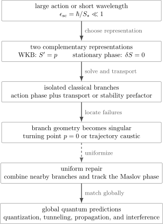
The two main routes share one logic. Classical action supplies the phase, transport or stability supplies the amplitude, and singular branch geometry requires a uniform approximation before global predictions are assembled.

What Is Actually Small?

Because $\hbar$ has units of action, the phrase “$\hbar$ is small” is incomplete. Choose a characteristic action $S_\star$ and define

$$\epsilon_{\mathrm{sc}} = \frac{\hbar}{S_\star}.$$

A semiclassical expansion requires $\epsilon_{\mathrm{sc}}\ll1$ for the observable, region, and time scale under study. The relevant action is not universal.

Local wave mechanics

If the momentum changes over a local scale

$$L_p(x) = \frac{\lvert p(x)\rvert}{\lvert p'(x)\rvert},$$

then

$$\epsilon_{\mathrm{WKB}}(x) = \frac{\hbar}{\lvert p(x)\rvert L_p(x)} = \left\lvert \hbar \frac{p'(x)}{p^2(x)} \right\rvert.$$

Equivalently,

$$\begin{aligned} \epsilon_{\mathrm{WKB}}(x) &= \frac{\lambda_{\mathrm{dB}}(x)} {2\pi L_p(x)}, \\ \lambda_{\mathrm{dB}}(x) &= \frac{2\pi\hbar} {\lvert p(x)\rvert}. \end{aligned}$$

The condition is local. A single state can be well described in one interval and badly described near a turning point, sharp interface, or singularity.

Bound motion

For a closed classical orbit, the natural action is

$$J(E) = \oint p\,dq.$$

Large quantum numbers often correspond to $J/\hbar\gg1$. This helps explain why action quantization becomes accurate high in a smooth spectrum, but it does not remove endpoint or separatrix corrections.

Propagation

For a trajectory joining fixed endpoints, the phase scale is the classical action

$$S_\gamma = \int_{t_i}^{t_f} L(q_\gamma,\dot q_\gamma,t)\,dt.$$

The ratio $\hbar/S_\gamma$ is only part of the story. Stationary points must also be isolated on the relevant scale, the fluctuation Hessian must be nondegenerate, and the amplitude and endpoints must be controlled. Large action does not make a caustic nonsingular.

One calculation can have several parameters

A tunneling problem can simultaneously involve:

• a small local WKB parameter away from the turning points;
• a large forbidden action $K/\hbar$ controlling exponential suppression;
• a turning-point scale controlling Airy matching;
• a barrier-top parameter that fails as two turning points approach.

Reporting only one global “semiclassical parameter” can hide the first place where the approximation fails.

WKB as Local Wave Mechanics

For a one-dimensional stationary Schrödinger equation,

$$\left[ - \frac{\hbar^2}{2m} \frac{d^2}{dx^2} + V(x) \right] \psi(x) = E\psi(x),$$

define the classical momentum in an allowed region by

$$p(x) = \sqrt{2m\bigl(E-V(x)\bigr)}.$$

The local phase obeys

$$S'(x)=\pm p(x),$$

which is the stationary Hamilton–Jacobi relation. The next equation transports the amplitude and gives $A\propto p^{-1/2}$. Thus, away from turning points,

Define the accumulated phase

$$\Theta(x) = \frac{1}{\hbar} \int^x p(x')\,dx'.$$

Then

$$\begin{aligned} \psi_{\mathrm{allow}}(x) &\approx \frac{1}{\sqrt{p(x)}} \\ &\quad\times \left[ C_+e^{i\Theta(x)} + C_-e^{-i\Theta(x)} \right]. \end{aligned}$$

The WKB Approximation derives this expansion and its transport equation. The present overview uses the result to show how local solutions become global predictions.

Why the amplitude is not optional

For one traveling branch, the probability current is

$$j = \frac{\hbar}{m} \operatorname{Im} \left( \psi^*\psi' \right).$$

To leading WKB order,

$$j_\pm \approx \pm \frac{\lvert C_\pm\rvert^2}{m}.$$

The factor $p^{-1/2}$ cancels the local momentum in the current. A constant-amplitude plane wave with changing $p(x)$ would not transport constant flux. For a standing-wave combination, the density envelope scales as $1/p(x)$, mirroring the greater classical dwell time where the particle moves slowly.

Forbidden regions

Where $V(x)\gt E$, define the positive momentum magnitude

$$\kappa(x) = \sqrt{2m\bigl(V(x)-E\bigr)}.$$

Define the accumulated forbidden-region action

$$\Xi(x) = \frac{1}{\hbar} \int^x\kappa(x')\,dx'.$$

The local branches are exponential:

$$\begin{aligned} \psi_{\mathrm{forbid}}(x) &\approx \frac{1}{\sqrt{\kappa(x)}} \\ &\quad\times \left[ D_+e^{\Xi(x)} + D_-e^{-\Xi(x)} \right]. \end{aligned}$$

“Growing” and “decaying” are orientation-dependent labels. A physical boundary condition selects the branch only after the integration direction and global geometry are stated. Between two turning points, both local branches can be needed during matching even when the final transmission is exponentially small.

Turning Points Are Part of the Method

A classical turning point $x_t$ satisfies

$$E=V(x_t), \qquad p(x_t)=0.$$

The leading WKB amplitude diverges there, and $\epsilon_{\mathrm{WKB}}$ cannot remain small. This is not a divergence of the exact wavefunction. It is evidence that the local branch coordinates have become singular.

For a simple turning point with $V'(x_t)\ne0$, linearize

$$V(x) \approx E+V'(x_t)(x-x_t).$$

The local Schrödinger equation reduces to the Airy equation on the length scale

$$\ell_t = \left( \frac{\hbar^2} {2m\lvert V'(x_t)\rvert} \right)^{1/3}.$$

Airy asymptotics overlap with WKB on both sides and supply the connection formula. This matched construction is a uniform repair: it remains finite through the region where the separate allowed and forbidden formulas fail.

Turning Points and Connection Formulas is the canonical home for the one-dimensional Airy matching and its factors of two and $\pi/4$ phases.

Not every turning point is simple

The Airy model assumes $V'(x_t)\ne0$ and an overlap region where both the linearized potential and WKB asymptotics are valid. Different local models are required when:

• two turning points coalesce near a barrier top;
• $V'(x_t)=0$ at a higher-order turning point;
• a singular endpoint replaces a smooth turning point;
• a hard wall imposes a boundary condition directly;
• the potential is discontinuous;
• several dimensions create a caustic rather than an isolated one-dimensional turn.

Connection formulas are therefore not decorative patches. Their local normal form must match the singular geometry.

From Local Solutions to Global Predictions

WKB is local, while spectra and scattering amplitudes are global. Boundary conditions and connection data assemble the local branches.

Bound-state quantization

For a smooth well with turning points $x_1(E)$ and $x_2(E)$, matching to decaying exterior tails gives

$$\begin{aligned} \int_{x_1}^{x_2} p(x;E)\,dx &= \pi\hbar \left( n+\frac{1}{2} \right), \\ n&=0,1,2,\ldots. \end{aligned}$$

Equivalently,

$$\oint p\,dx = 2\pi\hbar \left( n+\frac{1}{2} \right).$$

The shift is produced by two smooth turning points, not inserted as an empirical correction. Bohr–Sommerfeld Quantization owns the matching derivation and spectral checks. EBK Quantization generalizes the action rule to invariant tori in integrable systems.

Barrier penetration

For a smooth forbidden interval $x_1\lt x\lt x_2$, define

$$K(E) = \int_{x_1}^{x_2} \kappa(x;E)\,dx.$$

When $K/\hbar\gg1$, the leading transmission probability has the exponential structure

$$T(E) \sim \mathcal P(E) \exp\left[ - \frac{2K(E)}{\hbar} \right],$$

where $\mathcal P(E)$ is a prefactor determined by matching and scattering normalization. The exponent is often more robust than the prefactor, but it is not the whole answer near the barrier top or when accurate rates are required. See Barrier Penetration and Tunneling.

Phase bookkeeping

Turning points, focal points, and caustics change the phase of a semiclassical branch. The Maslov Index records these changes in a representation-independent way. Omitting it can preserve the magnitude while shifting nodes, spectra, and interference fringes.

Stationary Phase and Classical Trajectories

WKB starts from a differential equation. Semiclassical propagation starts from an oscillatory amplitude. The finite-dimensional prototype is

$$I(\hbar) = \int a(q) \exp\left[ \frac{i}{\hbar}S(q) \right]dq.$$

Away from stationary points, nearby contributions cancel under suitable smoothness and boundary assumptions. Near an isolated nondegenerate stationary point $q_\star$,

$$S'(q_\star)=0, \qquad S''(q_\star)\ne0,$$

the local quadratic expansion gives

$$\begin{aligned} I(\hbar) \sim{}& a(q_\star) \exp\left[ \frac{i}{\hbar}S(q_\star) \right] \\ &\times \exp\left[ i\frac{\pi}{4} \operatorname{sgn}S''(q_\star) \right] \sqrt{ \frac{2\pi\hbar} {\lvert S''(q_\star)\rvert} }. \end{aligned}$$

This formula already contains the semiclassical hierarchy: stationary action gives the leading phase, the Hessian gives the prefactor, and the Hessian signature gives an additional phase.

The rigorous hypotheses and multidimensional form belong to Asymptotic Analysis. Stationary Phase in Quantum Mechanics is the application guide for wave packets, propagator composition, partial-wave scattering, and saddle diagnostics. The regulated path-integral application belongs to Stationary Phase and the Classical Limit.

The Semiclassical Propagator

For fixed endpoints, stationary paths of the action satisfy

$$\delta S[q_\gamma]=0,$$

so they obey the classical Euler–Lagrange equations. The leading quantum propagator has the structure

$$\begin{aligned} K_{\mathrm{sc}} ={}& \sum_{\gamma:a\to b} \mathcal A_\gamma \\ &\times \exp\left[ \frac{i}{\hbar}S_\gamma - i\frac{\pi}{2}\nu_\gamma \right]. \end{aligned}$$

Each classical path contributes a complex amplitude, not a probability. Several paths can reach the same endpoint and interfere.

The prefactor is controlled by endpoint stability. In a standard coordinate convention,

$$\mathcal A_\gamma \propto \left\lvert \det\left( - \frac{\partial^2S_\gamma} {\partial q_b\,\partial q_a} \right) \right\rvert^{1/2}.$$

The Semiclassical Propagator gives the normalized formula, while the Van Vleck Determinant explains the stability geometry.

Caustics

At a caustic, the projection from a family of classical trajectories to endpoint configuration space becomes singular. The isolated-trajectory prefactor diverges even though the exact propagator remains a well-defined distribution. This is the multidimensional analogue of a WKB turning point. One must combine nearby branches into a uniform approximation and track the associated Maslov phase.

Quadratic actions as benchmarks

For a free particle and for a harmonic oscillator away from caustic times, the action is quadratic in fluctuations. The Gaussian stationary-phase calculation then terminates and gives the exact propagator after normalization. These cases are stronger than examples: they test every factor of $2\pi$, $i$, $\hbar$, and the determinant branch.

Phase Accuracy and Amplitude Accuracy

Semiclassical formulas are unusually sensitive to phase errors. If an approximate action is

$$S_{\mathrm{app}} = S+\delta S,$$

then the phase error is

$$\delta\phi = \frac{\delta S}{\hbar}.$$

An action can have a small relative error $\lvert\delta S/S\rvert$ while producing an order-one phase error when $S/\hbar$ is large. Long-time propagation, repeated orbits, and interference observables therefore demand more action accuracy than a smooth envelope may suggest.

Amplitude errors behave differently. A leading exponential tunneling estimate can capture orders of magnitude while missing an algebraic prefactor. Conversely, interference zeros can make a nominally subleading amplitude or phase correction dominate the observable.

A mature result distinguishes:

• phase order, including action and Maslov corrections;
• amplitude order, including transport and fluctuation determinants;
• uniformity, especially near turning points or caustics;
• global assembly, including boundary conditions and all comparable branches.

Pointwise and Uniform Validity

An approximation can be accurate at every fixed point away from a singular region and still fail as a global approximation. WKB near a turning point is the standard example: shrinking the forbidden or allowed distance with $\hbar$ enters a boundary layer where the leading outer expansion is not uniform.

The correct question is not only

$$\epsilon_{\mathrm{WKB}}(x)\ll1,$$

but also whether the observable samples regions where that condition fails. A bound-state normalization integral, a tunneling connection, or a propagator near a focal point can depend decisively on a small nonuniform region.

Matched and uniform approximations preserve the outer WKB description while replacing it locally. This is generally better than discarding semiclassics everywhere because it fails somewhere.

Benchmark Cases

Problem	What semiclassics teaches
Free particle	The stationary-phase propagator is exact because the action is quadratic.
Harmonic oscillator	Leading action quantization gives the exact energies, while turning-point matching remains essential for global wavefunctions.
Linear potential	Airy functions provide the exact local model of a simple turning point.
Smooth thick barrier	The forbidden action gives the dominant transmission exponent.
Rectangular step or barrier	Exact piecewise matching is natural; the abrupt interface violates slow variation even if the thick-barrier exponent resembles WKB.
Integrable multidimensional motion	EBK quantizes actions on invariant tori, with Maslov corrections.
Chaotic long-time motion	Local trajectory formulas can exist, but branch proliferation and instability restrict useful times and invalidate global EBK tori.

Exactness in a benchmark does not prove exactness in a neighboring problem. The free particle and oscillator are special because their relevant phase functions are quadratic.

Where Semiclassics Fails First

Turning points and caustics

The local momentum or fluctuation determinant vanishes. Use an Airy or another uniform normal form rather than an isolated branch.

Abrupt boundaries

The potential varies on a scale shorter than the wavelength. Use exact interface matching, or match WKB solutions to exact local boundary solutions away from the discontinuity.

Coalescing saddles

The Hessian degenerates and two isolated stationary contributions cease to be separable. A uniform approximation must keep both saddles together.

Separatrices and thresholds

Classical periods can diverge and action-angle coordinates can become singular. Ordinary quantization rules may require special threshold or separatrix analysis.

Long times and instability

Small errors in trajectories and actions can grow. In chaotic motion, the number of relevant branches can proliferate and the useful semiclassical time window can be much shorter than naive large-action counting suggests.

Complex or Euclidean saddles

Real classical trajectories do not describe every exponentially small amplitude. Tunneling can be represented by imaginary momentum in WKB or by complex and Euclidean saddles. These are controlled analytic continuations, not ordinary real-time classical paths under a forbidden barrier.

Low quantum numbers

Large action is least secure for the lowest few states. Some leading formulas remain exact in special solvable systems, but that success should be checked rather than generalized.

The cross-method Common Failure Modes guide organizes these breakdowns by symptom, test, and repair.

Relation to the Classical Limit

Semiclassical approximation and classical emergence are related but not identical.

• Stationary phase explains why classical equations organize leading contributions to amplitudes.
• It does not remove interference between several classical branches.
• WKB retains tunneling, which has no ordinary real classical trajectory.
• A narrow wave packet following a trajectory is a different approximation with its own spreading and time-scale conditions.
• Decoherence can suppress observable interference in a reduced state, but it is not supplied by stationary phase alone.
• The formal limit $\hbar\to0$ is shorthand for dimensionless action ratios; setting $\hbar=0$ inside the Schrödinger equation is singular.

The broader mechanisms are separated in Classical Limit and Common Misstatements About the Classical Limit. Semiclassical Limits and Correspondence gives this chapter’s practical contract for fixed-action limits, observable resolution, state classes, and time windows.

Method Roadmap

Question	Canonical page
How does classical action encode local quantum phase, momentum, energy, and rays?	Classical Action and Quantum Phase
How are the local phase, amplitude, and validity condition derived?	WKB Approximation
How are oscillatory WKB branches oriented, flux-normalized, and tested?	WKB in Classically Allowed Regions
How are evanescent WKB branches selected, interpreted, and tested?	WKB in Classically Forbidden Regions
What replaces WKB at a simple turning point?	Turning Points and Connection Formulas
How does matching quantize a smooth one-dimensional well?	Bohr–Sommerfeld Quantization
How is the dominant barrier transmission extracted?	Barrier Penetration and Tunneling
How does a repulsive Coulomb barrier produce alpha-decay and fusion energy scales?	Gamow Factor
How do eikonal phases, ray-tube amplitudes, and caustics generalize WKB?	Multidimensional WKB Preview
How is stationary phase applied to wave packets, composition, and high-energy scattering?	Stationary Phase in Quantum Mechanics
When should coherent states be propagated exactly, variationally, or as a trajectory sum?	Coherent-State Semiclassics Preview
How should a correspondence claim specify its parameter family, observables, resolution, and time window?	Semiclassical Limits and Correspondence
How are integrable multidimensional systems quantized?	EBK Quantization
Where do turning-point and caustic phase shifts live?	Maslov Index
How do classical paths approximate a propagator?	Semiclassical Propagator
How does classical stability determine the prefactor?	Van Vleck Determinant
What is the general action-over-$\hbar$ asymptotic framework?	Semiclassical Limit
How does stationary phase work in a regulated path integral?	Stationary Phase and the Classical Limit

Reporting Checklist

A semiclassical calculation should state:

1. Control parameter: the dimensionless action, wavelength, or saddle-separation ratio.
2. Region: allowed, forbidden, turning-point, caustic, boundary, or complex-saddle domain.
3. Order: phase, amplitude, and prefactor terms retained.
4. Boundary data: normalization, incoming or outgoing branches, endpoint conditions, and contour prescription.
5. Matching: how local solutions or trajectory branches are assembled.
6. Singular sets: turning points, caustics, thresholds, or separatrices and their local repairs.
7. Error evidence: next order, uniform estimate, exact benchmark, numerical comparison, or conservation check.
8. Observable: whether the claim concerns phase, energy, amplitude, probability, rate, or only exponential scaling.

Common Mistakes

• Calling energy “high” without checking a dimensionless local wavelength or action ratio.
• Treating $e^{iS/\hbar}$ as a probability weight rather than a phase.
• Keeping the action phase while dropping the transport prefactor and still claiming a normalized amplitude.
• Extending $p^{-1/2}$ through a turning point.
• Squaring an under-barrier amplitude but forgetting to double its exponent.
• Applying smooth-potential WKB at an abrupt interface.
• Using the two-turning-point $1/2$ shift for hard walls or singular endpoints.
• Summing probabilities instead of amplitudes when several classical paths contribute.
• Ignoring Maslov phases at caustics.
• Assuming a small relative action error guarantees a small phase error.
• Treating stationary phase as a complete explanation of decoherence or classicality.
• Calling an asymptotic formula convergent without evidence.

Exercises

1. Nondimensionalize a local wave equation

Suppose a region has characteristic momentum $p_\star$ and variation length $L$. Set $x=Ly$ and divide the stationary Schrödinger equation by $p_\star^2/(2m)$. Show that the coefficient of the second derivative is controlled by $\epsilon^2$, where $\epsilon=\hbar/(p_\star L)$.

Solution

Write the equation as

$$- \frac{\hbar^2}{2mL^2} \frac{d^2\psi}{dy^2} + V(Ly)\psi = E\psi.$$

Dividing by $p_\star^2/(2m)$ makes the derivative coefficient

$$\frac{\hbar^2}{p_\star^2L^2} = \epsilon^2.$$

The semiclassical limit is therefore a singularly perturbed second-order equation with a dimensionless small parameter, not a statement about the numerical value of dimensionful $\hbar$.

2. Flux and the WKB amplitude

For

$$\psi_+(x) = \frac{C}{\sqrt{p(x)}} \exp\left[ \frac{i}{\hbar} \int^x p(x')\,dx' \right],$$

show at leading WKB order that $j=\lvert C\rvert^2/m$.

Solution

The phase derivative supplies the leading term

$$\psi_+' \approx \frac{ip}{\hbar}\psi_+.$$

Hence

$$\begin{aligned} j &= \frac{\hbar}{m} \operatorname{Im} \left( \psi_+^*\psi_+' \right) \\ &\approx \frac{\hbar}{m} \operatorname{Im} \left( \frac{ip}{\hbar} \lvert\psi_+\rvert^2 \right) \\ &= \frac{p}{m} \frac{\lvert C\rvert^2}{p} = \frac{\lvert C\rvert^2}{m}. \end{aligned}$$

Derivatives of the slowly varying amplitude are subleading in the WKB ordering.

3. Divergence of the local validity parameter

Near a simple turning point, let $E-V(x)\approx F(x_t-x)$ on the allowed side, with $F\gt0$. Show that $\epsilon_{\mathrm{WKB}}$ diverges as $\lvert x-x_t\rvert^{-3/2}$.

Solution

The momentum behaves as

$$p(x) \approx \sqrt{2mF} \lvert x-x_t\rvert^{1/2}.$$

Therefore

$$\lvert p'(x)\rvert \approx \frac{\sqrt{2mF}}{2} \lvert x-x_t\rvert^{-1/2}.$$

Since $p^2\propto\lvert x-x_t\rvert$,

$$\epsilon_{\mathrm{WKB}} = \hbar \frac{\lvert p'\rvert}{p^2} \propto \lvert x-x_t\rvert^{-3/2}.$$

The failure is unavoidable arbitrarily close to the turning point, which is why Airy matching is part of the method.

4. Harmonic-oscillator action quantization

For a classical harmonic oscillator, the closed-orbit action is

$$J(E) = \frac{2\pi E}{\omega}.$$

Use the two-turning-point quantization rule to recover the quantum energies.

Solution

The smooth-well rule is

$$J(E_n) = 2\pi\hbar \left( n+\frac12 \right).$$

Substituting $J(E)=2\pi E/\omega$ gives

$$\frac{2\pi E_n}{\omega} = 2\pi\hbar \left( n+\frac12 \right),$$

so

$$E_n = \hbar\omega \left( n+\frac12 \right).$$

For this special quadratic system, the leading WKB spectrum is exact.

5. Interference of two classical paths

Two classical paths contribute equal prefactor magnitude $A$ and actions $S_1$ and $S_2$, with no additional relative Maslov phase. Compute the resulting probability factor and identify destructive interference.

Solution

The amplitude is

$$\mathcal M = A \left( e^{iS_1/\hbar} + e^{iS_2/\hbar} \right).$$

Therefore

$$\lvert\mathcal M\rvert^2 = 2\lvert A\rvert^2 \left[ 1+ \cos\left( \frac{S_1-S_2}{\hbar} \right) \right].$$

Destructive interference occurs when

$$S_1-S_2 = (2k+1)\pi\hbar, \qquad k\in\mathbb Z.$$

Adding the two path probabilities instead would miss this interference completely.

6. Relative action error versus phase error

A classical action satisfies $S/\hbar=10^4$. How small must the relative error $\lvert\delta S/S\rvert$ be to keep the phase error below $0.1$ radians?

Solution

The phase error is

$$\lvert\delta\phi\rvert = \frac{\lvert\delta S\rvert}{\hbar} = \frac{\lvert\delta S\rvert}{\lvert S\rvert} \frac{\lvert S\rvert}{\hbar}.$$

Requiring $\lvert\delta\phi\rvert\lt0.1$ gives

$$\frac{\lvert\delta S\rvert}{\lvert S\rvert} \lt \frac{0.1}{10^4} = 10^{-5}.$$

Thus a relative action error that looks small on an ordinary scale can still be too large for an interference-sensitive phase.

References

1. L. D. Landau and E. M. Lifshitz, Quantum Mechanics: Non-Relativistic Theory, 3rd ed. (Butterworth-Heinemann, 1981). Standard treatment of WKB wavefunctions, connection formulas, quantization, and tunneling.
2. C. M. Bender and S. A. Orszag, Advanced Mathematical Methods for Scientists and Engineers (Springer, 1999). Asymptotic expansions, WKB, turning points, and uniform approximations.
3. M. V. Berry and K. E. Mount, “Semiclassical approximations in wave mechanics”, Reports on Progress in Physics 35, 315–397 (1972). Broad review connecting WKB, turning points, phases, and multidimensional semiclassics.
4. V. P. Maslov and M. V. Fedoriuk, Semi-Classical Approximation in Quantum Mechanics (Reidel, 1981). Systematic treatment of canonical operators, caustics, and Maslov phases.
5. M. C. Gutzwiller, Chaos in Classical and Quantum Mechanics (Springer, 1990). Classical trajectories, propagators, periodic orbits, and quantum chaos.
6. M. Brack and R. K. Bhaduri, Semiclassical Physics (Westview Press, 2003). Graduate-level account of semiclassical quantization and applications.
7. L. S. Schulman, Techniques and Applications of Path Integration (Wiley, 1981). Path-integral stationary phase and semiclassical kernels.
8. F. W. J. Olver, Asymptotics and Special Functions (A K Peters, 1997). Rigorous asymptotics, turning points, and uniform expansions.