Stationary Phase in Quantum Mechanics

Stationary phase turns a rapidly oscillatory quantum integral into a sum of locally coherent contributions. Away from a stationary point, neighboring phases usually cancel. Near a nondegenerate stationary point, the phase changes only quadratically to leading order, so a neighborhood of width proportional to the inverse square root of the large parameter survives.

This page is an application and diagnostic guide. It does not duplicate the theorem or its full derivation. Stationary Phase is the canonical home for the one- and multidimensional formulas, Hessian signatures, and endpoint qualifications. Stationary Phase and the Classical Limit is the canonical regulated path-integral application.

The focus here is a different question:

when a quantum amplitude is presented as an oscillatory integral or sum, what is stationary, what physical object does the saddle select, and what invalidates the isolated-saddle answer?

Working Formula

Consider

$$I(\lambda) = \int_D d^n u\, a(u)e^{i\lambda\phi(u)},$$

where $\lambda\gg1$ is dimensionless. Let $u_s$ be isolated stationary points satisfying

$$\nabla\phi(u_s)=0,$$

with nonsingular Hessians

$$H_s = \left. \nabla\nabla\phi \right|_{u_s}, \qquad \det H_s\ne0.$$

When endpoint, contour, and support assumptions permit, the leading contribution is

$$\begin{aligned} I(\lambda) \sim{}& \left( \frac{2\pi}{\lambda} \right)^{n/2} \\ &\times \sum_s \frac{ a(u_s) e^{i\lambda\phi(u_s)} e^{i\pi\sigma_s/4} }{ \sqrt{\lvert\det H_s\rvert} }. \end{aligned}$$

Here $\sigma_s$ is the Hessian signature, the number of positive eigenvalues minus the number of negative eigenvalues.

In quantum mechanics, one often writes the phase as

$$\frac{\Phi(u)}{\hbar},$$

so the large dimensionless parameter is a characteristic action divided by $\hbar$. The stationary condition is

$$\nabla\Phi(u_s)=0.$$

The Hessian has units, and its determinant must be interpreted together with the integration measure and normalization. Writing “$\hbar\to0$” does not remove that dimensional bookkeeping.

What the Saddle Width Means

In one integration variable, expand near a nondegenerate saddle:

$$\phi(u) = \phi(u_s) + \frac12 \phi''(u_s) (u-u_s)^2 + \cdots.$$

The phase changes by order unity when

$$\lambda \lvert\phi''(u_s)\rvert (\Delta u)^2 \sim1.$$

Thus the contributing width scales as

$$\Delta u \sim \frac{1}{ \sqrt{ \lambda \lvert\phi''(u_s)\rvert } }.$$

This width is a diagnostic:

• the amplitude $a(u)$ should vary little across $\Delta u$;
• the saddle should remain well inside the integration domain on that scale;
• distinct saddles should be separated by more than their local widths;
• cubic and higher phase terms should be small over the same neighborhood.

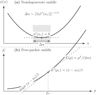
Left: a nondegenerate saddle contributes from a neighborhood $\Delta u\sim[\lambda\lvert\phi''(u_s)\rvert]^{-1/2}$. Right: for a freely propagating packet, stationarity means that the dispersion slope $dE/dp$ equals the observed displacement divided by time, selecting $p_s=m(x-x_0)/t$.

If $\phi''(u_s)=0$, this width estimate and the Gaussian formula both fail. The appropriate scaling is determined by the first nonzero higher derivative and usually requires a uniform approximation.

Saddle-Finding Workflow

For a quantum oscillatory integral, work in this order.

1. Isolate the full phase

Include phases carried by basis states, propagators, scattering matrices, boundary states, and the nominal amplitude. If

$$a(u) = \lvert a(u)\rvert e^{i\chi(u)}$$

and $\chi$ varies on the same rapid scale as $\Phi/\hbar$, then $\chi$ belongs in the stationary phase:

$$\Phi_{\mathrm{tot}}(u) = \Phi(u) + \hbar\chi(u).$$

Treating a rapidly varying factor as a “slow amplitude” moves the saddle and can change the answer qualitatively.

2. Identify the large parameter

The large parameter may be:

• action divided by $\hbar$;
• propagation distance divided by wavelength;
• time times an energy-curvature scale divided by $\hbar$;
• angular momentum $\ell\gg1$;
• a large particle number or other dimensionless semiclassical scale.

State it explicitly. A large dimensional number by itself is not an asymptotic parameter.

3. Solve the stationary equations with boundary data

Find every relevant real or complex solution of

$$\nabla\Phi=0$$

that is compatible with the integration domain and contour. A formal solution outside the amplitude support or on an inaccessible steepest-descent contour does not contribute in the same way as an interior real saddle.

4. Classify each contribution

Check:

$$\det H_s,$$

the Hessian signature, distance to endpoints, singularities of $a$, contour orientation, and separation from other saddles.

5. Sum amplitudes before probabilities

When several saddles contribute coherently,

$$\mathcal A \sim \sum_s\mathcal A_s.$$

The observable contains interference terms. Stationary phase does not turn a coherent quantum sum into a classical mixture.

6. Estimate the neglected structure

Test amplitude variation, higher phase derivatives, endpoint terms, and any deformation used to reach complex saddles. Numerical comparison against the original integral is often inexpensive and highly informative.

Free Wave-Packet Propagation

Use the convention

$$\langle x\mid p\rangle = \frac{1}{\sqrt{2\pi\hbar}} e^{ipx/\hbar}.$$

Suppose a packet initially localized near $x_0$ has momentum wavefunction

$$\widetilde\psi(p,0) = a(p)e^{-ipx_0/\hbar},$$

where $a(p)$ is slowly varying on the stationary-phase scale. Its free evolution is

$$\psi(x,t) = \frac{1}{\sqrt{2\pi\hbar}} \int_{-\infty}^{\infty} dp\, a(p) e^{i\Phi(p;x,t)/\hbar},$$

with

$$\Phi(p;x,t) = p(x-x_0) - E(p)t.$$

The stationary condition is

$$\frac{\partial\Phi}{\partial p} = x-x_0 - t\frac{dE}{dp} = 0.$$

Therefore the contributing momentum satisfies

$$\frac{x-x_0}{t} = v_{\mathrm g}(p_s),$$

where

$$v_{\mathrm g} = \frac{dE}{dp}.$$

Stationary phase selects the momentum component whose group velocity carries it from $x_0$ to $x$ in time $t$.

Free quadratic dispersion

For

$$E(p) = \frac{p^2}{2m},$$

the saddle is

$$p_s = \frac{m(x-x_0)}{t}.$$

The phase curvature and saddle action are

$$\begin{aligned} \Phi''(p_s) &= - \frac{t}{m}, \\ \Phi(p_s) &= \frac{ m(x-x_0)^2 }{2t}. \end{aligned}$$

For $t\gt0$ and an interior saddle,

$$\begin{aligned} \psi(x,t) \sim{}& \sqrt{\frac{m}{t}}\, a(p_s) \\ &\times \exp\left[ \frac{ im(x-x_0)^2 }{2\hbar t} - \frac{i\pi}{4} \right]. \end{aligned}$$

Consequently,

$$\lvert\psi(x,t)\rvert^2 \sim \frac{m}{t} \lvert a(p_s)\rvert^2.$$

This is the one-dimensional time-of-flight map: at long propagation time, position resolves the initial momentum distribution through $p_s=m(x-x_0)/t$. It is an asymptotic statement, not an assertion that a finite-width packet follows one exact trajectory.

If $p_s$ lies outside the effective support of $a(p)$, the interior saddle estimate does not apply. Tails, endpoints, or complex saddles may then control the result.

Propagator Composition

The exact composition law is

$$\begin{aligned} K(q_f,t_f;q_i,t_i) ={}& \int dq\, K(q_f,t_f;q,t) \\ &\times K(q,t;q_i,t_i). \end{aligned}$$

Suppose each kernel is approximated by a semiclassical branch with actions

$$S_2(q_f,t_f;q,t)$$

and

$$S_1(q,t;q_i,t_i).$$

The intermediate-coordinate phase is

$$\Phi(q) = S_2(q_f,t_f;q,t) + S_1(q,t;q_i,t_i).$$

Stationarity requires

$$\frac{\partial\Phi}{\partial q} = 0.$$

Endpoint derivatives of the classical action give

$$\begin{aligned} \frac{\partial S_1}{\partial q} &= p_{\mathrm{in}}, \\ \frac{\partial S_2}{\partial q} &= - p_{\mathrm{out}}. \end{aligned}$$

Therefore

$$p_{\mathrm{in}} = p_{\mathrm{out}}.$$

The saddle glues two classical segments into one differentiable classical trajectory. The Gaussian determinant supplies the composition prefactor. Semiclassical Propagator and Van Vleck Determinant own the complete formula and its stability interpretation.

Classical Equations from Stationary Action

For a path integral, the integration variable is an entire history rather than one momentum or intermediate coordinate. Formally,

$$\mathcal A \sim \int\mathcal Dq\, e^{iS[q]/\hbar}.$$

The stationary condition

$$\delta S[q_{\mathrm{cl}}]=0$$

gives the Euler–Lagrange equations with the boundary conditions of the amplitude being computed.

This statement must be regulated before determinants and powers of $\hbar$ are manipulated. The exact path integral still includes nonstationary histories; the saddle expansion reorganizes their collective contribution. The detailed time-sliced derivation belongs to Stationary Phase and the Classical Limit.

Partial-Wave Scattering

For a central potential, elastic scattering uses

$$S_\ell = e^{2i\delta_\ell}.$$

At high energy or large angular momentum, a partial-wave sum may be approximated by an integral over continuous $\ell$. After the large-$\ell$ angular function is decomposed into two traveling angular branches, the relevant phases have the schematic form

$$\Phi_\pm(\ell) = 2\delta_\ell \pm \left( \ell+\frac12 \right)\theta.$$

Stationarity gives

$$2 \frac{d\delta_\ell}{d\ell} \pm \theta = 0.$$

Define the semiclassical deflection function in this phase convention by

$$\Theta(\ell) = 2 \frac{d\delta_\ell}{d\ell}.$$

Then the partial waves contributing to angle $\theta$ satisfy

$$\Theta(\ell_s) = \mp\theta.$$

The sign is tied to the chosen angular traveling-wave branch and deflection convention. It should be stated rather than guessed.

Using

$$b \approx \frac{\ell+1/2}{k},$$

the saddle connects angular momentum to a classical impact parameter. Several solutions $\ell_s$ at one angle produce semiclassical interference.

Rainbow scattering

A rainbow occurs at an extremum of the deflection function:

$$\left. \frac{d\Theta}{d\ell} \right|_{\ell_r} = 0.$$

At the corresponding angle,

$$\Phi_\pm''(\ell_r)=0.$$

Two ordinary scattering saddles coalesce, and the nondegenerate stationary-phase amplitude diverges. An Airy uniform approximation replaces the separate saddle terms and gives a finite wave pattern with oscillatory supernumerary structure.

Partial-Wave Expansion owns the exact quantum expansion and phase-shift conventions. This section only explains the additional semiclassical saddle interpretation.

QFT Saddle-Point Bridge

In quantum field theory, the analogous formal object is

$$Z = \int\mathcal D\phi\, e^{iS[\phi]/\hbar}.$$

A saddle $\phi_s$ satisfies

$$\left. \frac{\delta S}{\delta\phi} \right|_{\phi_s} = 0.$$

Expanding around $\phi_s$ produces:

• the classical action in the leading phase;
• a functional determinant from quadratic fluctuations;
• interaction vertices from higher variations;
• sums over several saddles when more than one contributes.

The finite-dimensional analogy is useful but incomplete. QFT saddle expansions may require gauge fixing, ghosts, collective coordinates, regularization, renormalization, boundary counterterms, and a specified contour or $i\epsilon$ prescription. A formal solution of the classical field equation is not automatically a contributing saddle.

Contributions Beyond Interior Saddles

Stationary points are not the only source of asymptotic contributions.

Endpoints and boundaries

If the integration domain ends before a stationary point is reached, integration by parts often produces endpoint terms. Their scaling can differ from the Gaussian $\lambda^{-1/2}$ law.

Poles and branch points

Contour deformation may cross a pole or wrap a branch cut. Residues or discontinuities can dominate over real-axis saddles.

Complex saddles

Tunneling, decay, and steepest-descent problems frequently require complex stationary points. Whether they contribute depends on the integration contour and its allowed deformation, not only on the equation $\nabla\Phi=0$.

Stationary manifolds and zero modes

If a continuous symmetry generates a family of saddles, the Hessian has zero modes. One should introduce collective coordinates and integrate along the stationary manifold rather than divide by a zero determinant.

Coalescing saddles

When saddle separation becomes comparable to the local saddle width, isolated Gaussian terms are not uniform. Fold coalescence gives Airy behavior; other degeneracies require other canonical integrals.

Rapid or singular amplitudes

A pole, cusp, hard cutoff, or rapidly varying phase hidden inside $a(u)$ invalidates the assumption that the amplitude is locally constant over the saddle region.

Stationary Phase Is Not Decoherence

Stationary phase explains cancellation in an amplitude integral. It does not by itself:

• remove nonstationary alternatives from the exact theory;
• select one saddle when several contribute;
• convert a coherent saddle sum into a probability mixture;
• explain why macroscopic records are stable;
• produce environmental decoherence.

Several saddles can remain coherent and generate strong interference. Classical-looking trajectories inside an approximation are not the same as an emergent classical stochastic description.

Which Canonical Page to Use

Need	Canonical page
One- and multidimensional stationary-phase theorem	Stationary Phase
Regulated path-integral saddle derivation	Stationary Phase and the Classical Limit
Action phases and local classical momentum	Classical Action and Quantum Phase
Eikonal rays, transport, and caustics	Multidimensional WKB Preview
Propagator branch sum	Semiclassical Propagator
Stability prefactor	Van Vleck Determinant
Exact central-potential partial-wave sum	Partial-Wave Expansion
Path-integral bridge to field theory	Path Integrals

Common Mistakes

• Calling a dimensional quantity “large” without forming a dimensionless phase parameter.
• Differentiating only the obvious exponential while ignoring a rapid phase in the amplitude.
• Keeping a stationary point outside the integration domain or amplitude support.
• Using the Gaussian formula when the Hessian determinant vanishes.
• Ignoring endpoint, pole, branch-cut, or contour contributions.
• Keeping only one saddle when several have comparable size.
• Adding saddle probabilities instead of coherent saddle amplitudes.
• Treating a real classical solution as a contributing QFT saddle without checking the contour.
• Using the partial-wave deflection function without declaring its sign convention.
• Interpreting a rainbow divergence as physical rather than as failure of isolated saddles.
• Claiming stationary phase alone explains decoherence or the full classical limit.

Reporting Checklist

A stationary-phase estimate should state:

1. the original integral or regulated sum;
2. the complete phase and amplitude;
3. the dimensionless large parameter;
4. all relevant saddles and their domain or contour status;
5. the Hessian determinant and signature convention;
6. endpoint, singularity, and complex-contour contributions;
7. saddle separation and any uniform approximation;
8. the first neglected scale or a numerical comparison;
9. whether saddle amplitudes remain coherent.

Exercises

1. Gaussian benchmark

Evaluate exactly

$$I(\lambda) = \int_{-\infty}^{\infty} \exp\left( - \frac{x^2}{2} \right) \exp\left( \frac{i\lambda x^2}{2} \right) \,dx$$

and compare its large-$\lambda$ behavior with stationary phase.

Solution

Combine the exponents:

$$I(\lambda) = \int_{-\infty}^{\infty} \exp\left[ - \frac12 (1-i\lambda)x^2 \right] \,dx.$$

Since the real part of $1-i\lambda$ is positive,

$$I(\lambda) = \sqrt{ \frac{2\pi}{1-i\lambda} },$$

with the square root chosen continuously from $\lambda=0$.

For $\lambda\to+\infty$,

$$1-i\lambda \sim \lambda e^{-i\pi/2},$$

so

$$I(\lambda) \sim \sqrt{ \frac{2\pi}{\lambda} } e^{i\pi/4}.$$

The phase is stationary at $x_s=0$, where $\phi''(0)=1$ and the amplitude equals $1$. The one-dimensional stationary-phase formula gives the same result.

2. Free-packet saddle

Starting from

$$\psi(x,t) = \frac{1}{\sqrt{2\pi\hbar}} \int dp\, a(p) e^{i\Phi(p)/\hbar},$$

where

$$\Phi(p) = p\Delta x - \frac{p^2t}{2m},$$

with $\Delta x=x-x_0$ and $t\gt0$, find the leading stationary-phase approximation.

Solution

The phase is

$$\Phi(p) = p\Delta x - \frac{p^2t}{2m}.$$

Stationarity gives

$$\Phi'(p_s) = \Delta x - \frac{p_st}{m} = 0,$$

so

$$p_s = \frac{m\Delta x}{t}.$$

At the saddle,

$$\Phi(p_s) = \frac{m(\Delta x)^2}{2t}, \qquad \Phi''(p_s) = - \frac{t}{m}.$$

The Gaussian factor is

$$\sqrt{ \frac{2\pi\hbar m}{t} } e^{-i\pi/4}.$$

After multiplying by the Fourier normalization,

$$\begin{aligned} \psi(x,t) \sim{}& \sqrt{\frac{m}{t}}\, a(p_s) \\ &\times \exp\left[ \frac{ im(\Delta x)^2 }{2\hbar t} - \frac{i\pi}{4} \right]. \end{aligned}$$

3. Momentum matching in composition

For the phase

$$\Phi(q) = S_2(q_f,t_f;q,t) + S_1(q,t;q_i,t_i),$$

show that stationarity in $q$ matches the momenta of the two classical segments.

Solution

For the first segment, $q$ is the final endpoint, so

$$\frac{\partial S_1}{\partial q} = p_{\mathrm{in}}.$$

For the second segment, $q$ is the initial endpoint, so

$$\frac{\partial S_2}{\partial q} = - p_{\mathrm{out}}.$$

Therefore

$$\frac{\partial\Phi}{\partial q} = p_{\mathrm{in}} - p_{\mathrm{out}}.$$

The saddle equation gives

$$p_{\mathrm{in}} = p_{\mathrm{out}}.$$

The composed path has continuous canonical momentum at the intermediate point.

4. Endpoint contribution without a saddle

Evaluate

$$I(\lambda) = \int_0^1 \, e^{i\lambda x}\,dx$$

and explain why “no stationary point” does not mean “zero asymptotic contribution.”

Solution

Direct integration gives

$$I(\lambda) = \frac{ e^{i\lambda}-1 }{ i\lambda }.$$

The phase derivative is constant:

$$\phi'(x)=1,$$

so there is no interior saddle. Nevertheless,

$$I(\lambda)=O(\lambda^{-1}).$$

The two terms come from the endpoints. Nonstationary interior regions cancel strongly, but boundaries remain and must be included in the asymptotic analysis.

5. Degenerate scaling

Consider a regulated integral localized near $x=0$ with phase

$$\lambda\frac{x^3}{3}.$$

Use a rescaling to determine the saddle width and leading power of $\lambda$.

Solution

The saddle at $x=0$ is degenerate:

$$\begin{aligned} \phi'(0)&=0, \\ \phi''(0)&=0, \\ \phi'''(0)&\ne0. \end{aligned}$$

Set

$$x = \lambda^{-1/3}y.$$

Then

$$\lambda\frac{x^3}{3} = \frac{y^3}{3}, \qquad dx = \lambda^{-1/3}dy.$$

Thus the contributing width scales as

$$\Delta x \sim \lambda^{-1/3},$$

and the leading integral scales as $\lambda^{-1/3}$, not $\lambda^{-1/2}$. The ordinary Gaussian formula cannot be used because its denominator contains $\sqrt{\lvert\phi''(0)\rvert}=0$.

6. Scattering saddle and rainbow

Take

$$\Phi_\pm(\ell) = 2\delta_\ell \pm \left( \ell+\frac12 \right)\theta.$$

Derive the saddle condition and show why an extremum of the deflection function is a degenerate saddle.

Solution

Differentiate:

$$\Phi_\pm'(\ell) = 2 \frac{d\delta_\ell}{d\ell} \pm \theta.$$

With

$$\Theta(\ell) = 2 \frac{d\delta_\ell}{d\ell},$$

the saddle condition is

$$\Theta(\ell_s) = \mp\theta.$$

The phase curvature is

$$\Phi_\pm''(\ell) = \frac{d\Theta}{d\ell}.$$

At a rainbow,

$$\left. \frac{d\Theta}{d\ell} \right|_{\ell_r} = 0,$$

so the saddle Hessian vanishes. Two angular-momentum saddles coalesce, the isolated Gaussian contributions are not uniform, and an Airy approximation is required.

References

1. R. Wong, Asymptotic Approximations of Integrals, 2nd ed. (SIAM, 2001). Stationary phase, endpoints, coalescing saddles, and uniform asymptotics.
2. N. Bleistein and R. A. Handelsman, Asymptotic Expansions of Integrals (Dover, 1986). Systematic steepest-descent and stationary-phase methods.
3. M. V. Berry and K. E. Mount, “Semiclassical approximations in wave mechanics”, Reports on Progress in Physics 35, 315–397 (1972). Quantum applications, caustics, and semiclassical branches.
4. K. W. Ford and J. A. Wheeler, “Semiclassical description of scattering”, Annals of Physics 7, 259–286 (1959). Deflection functions, interference, rainbows, glories, and orbiting.
5. R. G. Littlejohn, “The semiclassical evolution of wave packets”, Physics Reports 138, 193–291 (1986). Wave-packet and phase-space semiclassics.
6. M. C. Gutzwiller, Chaos in Classical and Quantum Mechanics (Springer, 1990). Classical paths, stationary phase, stability, and trace formulas.
7. L. S. Schulman, Techniques and Applications of Path Integration (Wiley, 1981). Path-integral stationary phase and semiclassical kernels.
8. R. G. Newton, Scattering Theory of Waves and Particles, 2nd ed. (Springer, 1982). Partial waves and semiclassical scattering.