Noise, Channels, and Error Mitigation

A noisy quantum-information claim is a chain from an intended task to an observed record, not merely the name of a channel. This guide supplies a model-to-decision workflow for freezing the physical and computational boundary, distinguishing mechanisms from representations, recording preparation, process, measurement, context, memory, and drift assumptions, and auditing the evidence and total cost of any proposed intervention. Its exit capability is practical: given a device discrepancy, fitted noise model, mitigation result, or scalability claim, a reader can identify what has actually been established and route every specialist question to its canonical owner.

The guide compares and checks; it does not rederive channel-representation theorems, microscopic reduced dynamics, specialist mitigation protocols, or error-correction constructions. Its organizing question is: What physical or operational discrepancy is being modeled, under which preparation–process–measurement and context assumptions, with what evidence, intervention, uncertainty, and total cost? The answer must remain meaningful when the same data admit several models, when a calibration becomes stale, or when a lower overhead in one currency creates a larger cost in another.

Required background. Circuit Model supplies preparation–operation–measurement records, circuit locations, classical outcomes, causal execution, and logical resource currencies. Quantum Channels and Noise supplies completely positive trace-preserving maps, conditional instruments, channel composition, and the conventions needed to read Kraus, Choi, affine, and superoperator descriptions.

Helpful background. Density Operators for Quantum Information supplies state, ensemble, reduced-state, and subnormalized-branch bookkeeping. Mathematical Toolkit Variance and Covariance supplies estimator variance, covariance propagation, and uncertainty calculations used when several noisy estimates are combined.

Noise and Mitigation as a Model-to-Decision Layer

Freeze a claim before choosing a channel

Begin with the discrepancy rather than a favorite formula. State the intended preparation, operation, measurement, or output distribution; identify the circuit location and time window; and record what was observed. A Ramsey contrast decay, an unexpected population, a conditional shift during a neighboring gate, and a biased readout histogram are distinct observations. Each can sometimes be reproduced by several mathematical models, and none alone identifies a microscopic cause.

For an input label $x$, outcome $y$, acquisition time $t$, and circuit context $c$, the operational probability is

$$p(y\mid x,t,c) = \operatorname{Tr}\!\left[ M_{y,t,c}\, \mathcal E_{t,c}\!\left(\rho_{x,t,c}\right) \right].$$

The same change in $p(y\mid x,t,c)$ can be assigned to the prepared state $\rho_{x,t,c}$, the process $\mathcal E_{t,c}$, the measurement effect $M_{y,t,c}$, or a combination. Time and context can alter all three. A fitted map is therefore evidence within a declared experiment design, not an identification theorem and not automatically a transferable device property.

A frozen claim names the target estimand as well. Estimating one Hamiltonian expectation, sampling an entire bit-string distribution, preserving an unknown state, and obtaining an accepted symmetry sector are different tasks. An intervention can improve one while degrading another. Only after the task, system boundary, data, and acceptance condition are fixed is it sensible to choose a channel family, diagnostic, or mitigation rule.

What this guide owns

This guide owns the transitions between layers: discrepancy to mechanism hypothesis; mechanism hypothesis to a deliberately limited representation; representation to diagnostic and calibration data; fitted model to held-out or workload validation; validated model to control, mitigation, correction, or no intervention; and intervention to accepted-answer cost and a new validation obligation.

The mathematical equivalence of channel representations remains with the open-systems owners. Choi and Stinespring support that formal foundation; their theorems are not reproduced here. Likewise, the generator results of Gorini, Kossakowski, and Sudarshan and Lindblad belong to the theory of quantum dynamical semigroups, not to a device-facing shortcut from an exponential fit to a universal noise law.

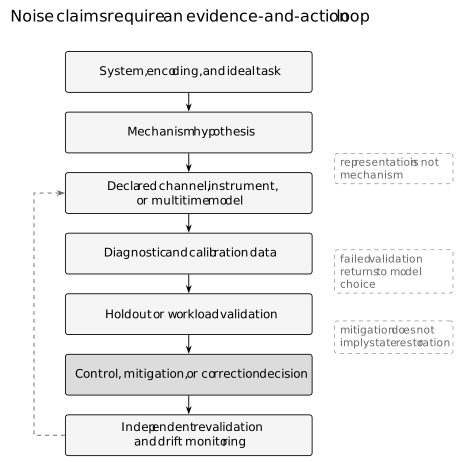
Evidence moves from a declared system and task through a mechanism hypothesis, representation, diagnostic data, held-out validation, intervention, and independent revalidation. Representation is not mechanism, mitigation does not imply state restoration, and failed validation returns the analysis to model choice.

The loop is intentionally recurrent. Calibration and mitigation can change pulse schedules, duration, measurement balance, or retained data, thereby changing the effective process. A model that supported yesterday’s intervention must be rechecked in the context in which today’s conclusion will be used.

The Ten-Field Noise-to-Action Record

Record fields in declared order

Use the following record for every worked claim. A field may be N/A only when the quantity genuinely does not apply; unknown, not measured, assumed fixed, and excluded from the boundary are informative and must not be replaced by N/A.

Field	Required record
1	System, encoding, retained sectors, and trusted boundary.
2	Ideal preparation, process, measurement, and circuit location.
3	Task, estimand or output, and acceptance condition.
4	Physical mechanism hypothesis.
5	Mathematical representation and parameter convention.
6	Time resolution, spatial/context scope, memory, and stationarity window.
7	Data, diagnostic, calibration, and identifiability assumptions.
8	Intervention: control, mitigation, detection, correction, or none.
9	Bias/error, variance/confidence, and success or acceptance probability.
10	Attempts, shots, recalibration, classical work, validation, and canonical owner.

The first three fields define what an error could mean. Fields four and five keep a physical story separate from a computational representation. Fields six and seven delimit when the representation is predictive. Fields eight through ten turn a model into an auditable action rather than an attractive fit. Record the fields before examining a favorable mitigated answer; otherwise the analysis can silently adapt its boundary, metric, or excluded costs to the result.

For a circuit experiment, the ideal operation should include idles, resets, measurements, classical conditions, and discarded branches when those affect the task. For a logical calculation, the system boundary should say whether leaked levels, photons that were lost, rejected shots, or decoder failures remain inside the accounting. For a claimed device parameter, the stationarity window should name the calibration epoch and contexts in which the estimate was tested.

Mechanism, representation, evidence, and action

A mechanism is a physical or operational hypothesis such as detuning, energy exchange, a spectator interaction, detector misclassification, or a drifting control parameter. A representation is a mathematical object such as a channel, instrument, stochastic process, affine map, transfer matrix, or multitime process tensor. Evidence consists of data and a diagnostic design capable of distinguishing relevant alternatives. An action is a control update, estimator transformation, rejection rule, encoded correction, or decision to collect different data.

These four nouns should never be collapsed. Amplitude damping can be a useful representation of relaxation without identifying the microscopic bath. A Pauli channel can predict selected syndrome statistics without proving that physical faults occur as classical Pauli events. A positive Choi matrix certifies complete positivity under the declared convention; it does not certify stationarity or locality. Conversely, a plausible microscopic mechanism is not yet a quantitative model of a compiled workload.

The record makes the inferential direction visible. A channel fitted to calibration circuits becomes evidence for a workload only through validation circuits not used to select the model. A mitigation rule becomes evidence for improved accuracy only when the ideal target is known independently or bounded on held-out instances. A lower variance is not a lower bias, and a lower conditional error after rejection is not automatically a lower cost per accepted answer.

Freeze the System Boundary and Ideal Task

Device, encoding, and retained sectors

The physical device usually has more degrees of freedom than the logical description. A transmon called a qubit has higher levels; a photonic encoding can lose a carrier; a bosonic code occupies a subspace of a mode; and a multiqubit processor includes spectators, couplers, controls, and classical electronics. Let $P$ project onto the retained computational or code subspace. For a state initially inside that subspace, one operational leakage probability is

$$L_{\mathcal E}(\rho) = \operatorname{Tr}\!\left[ (I-P)\mathcal E(\rho) \right].$$

This number depends on $P$, the input ensemble, and the time or circuit location. It does not describe what happens after leakage, whether population returns, whether the event is detected, or whether leaked population harms a neighbor. Wood and Gambetta distinguish leakage and seepage and show why average gate fidelity alone is incomplete for an encoded subspace.

Loss and leakage should also be separated from erasure. An erasure is flagged in an orthogonal record available to the protocol. Unflagged photon loss or population outside a detector’s modeled outcomes need not supply that information. Postselecting on a herald changes the retained ensemble and introduces an acceptance cost; it does not turn every loss mechanism into a cost-free erasure.

Ideal operation and circuit location

Name the ideal object at the level on which the conclusion is made. For a gate location it may be a unitary channel $\mathcal U(\rho)=U\rho U^\dagger$. For an idle it may be the identity in a specified rotating frame. For readout it is an instrument with both probabilities and conditional states, not only a classical label. For a complete algorithm it includes preparation, routing, feedforward, measurement, retries, and classical postprocessing.

Frame conventions matter. A deterministic $Z$ phase can be a coherent error in one frame, an intentional virtual-frame update in another, or an irrelevant phase for a restricted terminal measurement. Likewise, placing a channel before a gate is generally not equivalent to placing it after:

$$\mathcal E\circ\mathcal U \ne \mathcal U\circ\mathcal E.$$

The record must state the placement rather than drawing an unlabeled noise symbol. Gate-local, cycle-local, and end-of-circuit models support different predictions. A model fitted to isolated gates does not automatically describe simultaneous gates, idles inserted by scheduling, or measurement activity.

Estimand, output, and acceptance

The estimand is the quantity the data analysis seeks to infer. Examples include an expectation $\mu=\operatorname{Tr}(O\rho)$, an outcome probability, a fidelity-like average, a logical failure probability per cycle, or a cost-to-solution at fixed quality and confidence. State restoration is a stronger task than estimating a selected expectation; sampling a distribution is different from estimating several of its moments.

Write the acceptance condition before mitigation. If an estimate $\widehat\mu$ must satisfy

$$\Pr\!\left( |\widehat\mu-\mu_0|\le\epsilon \right) \ge 1-\delta,$$

then $\mu_0$, $\epsilon$, $\delta$, the probability source, and any bias allowance must be declared. A root-mean-square error, a confidence interval with frequentist coverage, and a Bayesian credible interval answer related but distinct questions. If only accepted shots enter the estimator, say whether $\mu_0$ refers to the unconditional ideal experiment or to a conditional sector.

This discipline prevents a common category error: showing that a mitigated number moved toward a reference on one tractable instance and then claiming that the underlying state was corrected. The evidence licenses the stated estimand on the validated domain—no more and no less.

Separate Mechanisms from Representations

Mechanism hypotheses are not fitted matrices

A coherent overrotation, stochastic control fluctuation, Markovian decay, quasistatic detuning, leakage event, and readout misclassification may all alter a finite data set. The mechanism hypothesis asks which degrees of freedom and causal couplings could produce the discrepancy. The fitted matrix asks which input–output transformation summarizes the chosen experiments. Agreement between them requires additional evidence.

For example, an apparently dephasing channel can arise from entanglement with an environment, averaging a slowly varying coherent detuning over shots, averaging unresolved spatial inhomogeneity, or deliberately randomized control. These mechanisms predict different behavior under echo, changed acquisition ordering, faster sampling, or an enlarged system boundary. A useful diagnostic changes one of those conditions and tests the resulting prediction.

The same caution applies in reverse. A microscopic narrative about flux noise or thermal photons does not specify a channel parameter, time dependence, or circuit placement. Mechanism claims need an observation model, and channel claims need a domain of validity.

Coherent, stochastic, dissipative, and thermal mechanisms

Coherent miscalibration implements the wrong reversible transformation on the retained system. Repeating an aligned error can add amplitudes before probabilities are formed. A stochastic mixture averages different transformations and may accumulate differently even when a one-step average infidelity is matched. Dissipative dynamics exchanges energy or information with degrees of freedom outside the retained description. Thermal exchange includes both downward and upward transitions and approaches a temperature-dependent fixed point rather than necessarily $|0\rangle$.

These categories overlap at different resolutions. Slow classical noise looks coherent during one shot and stochastic across an ensemble. A driven multilevel device can show coherent leakage followed by dissipative return. Randomized compiling can turn selected coherent structure into an effective stochastic description for designated observables, but the resulting Pauli model is still a justified approximation, not a declaration of the underlying microscopic events.

Relaxation and dephasing times are model summaries. The familiar relation

$$\frac{1}{T_2} = \frac{1}{2T_1} + \frac{1}{T_\phi}$$

assumes a restricted weak-coupling, exponential, two-level model with separable pure dephasing. It is not a definition for driven, nonexponential, multilevel, or memory-bearing dynamics. A gate much shorter than $T_1$ can still be limited by control error, crosstalk, or leakage.

Leakage, loss, crosstalk, and SPAM

Leakage changes the retained sector. Loss removes or relocates a carrier. Crosstalk means that the operation or observation at one location depends on activity or state elsewhere in a way excluded by the nominal local model. SPAM collects state-preparation and measurement discrepancies, but that label does not make those components separately identifiable.

Sarovar and collaborators formulate operational tests for crosstalk, while Rudinger and collaborators show how pooled circuit data can reveal context dependence and drift. Their results motivate testing spectator state, simultaneous operations, acquisition epoch, and other context variables. Correlated errors are not automatically crosstalk: two qubits may share a bath even when neither control acts directly on the other. Conversely, crosstalk can produce a deterministic coherent shift rather than a random correlated fault.

Mechanism	Representation	Signature	Diagnostic or falsifier	Owner or action
coherent miscalibration	unitary offset or Hamiltonian term	phase-sensitive, potentially aligned accumulation	amplify with repeated gates and vary axes or frames	calibrate control; validate in workload
relaxation or dephasing	nonunital or coherence-contraction channel	population or off-diagonal decay versus time	compare inversion recovery, Ramsey, and echo under declared fits	choose a time- and basis-aware model
stochastic Pauli noise	Pauli mixture or transfer eigenvalues	axis-dependent probabilistic contraction	prepare several axes and test multi-step prediction	use only after structure and convention checks
leakage or loss	enlarged-space channel or flagged branch	missing retained-sector population	measure outside the code space and test return or heralding	retain leakage, seepage, and acceptance costs
crosstalk	context-dependent joint map or Hamiltonian	outcome changes with spectator or simultaneous activity	randomize contexts and test conditional dependence	localize context before calibration or scheduling
SPAM	preparation states plus measurement effects	short-sequence bias shared across gate estimates	add fiducials, trusted references, or self-consistent designs	report gauge and identifiability limits
temporal memory	multitime process or latent history variable	later outcomes depend on interventions or earlier records	permute sequences, insert causal breaks, vary delays	enlarge the model or shorten its validity window
spatial or context correlation	joint fault law or context-dependent channel	factorized model fails on joint or simultaneous data	compare isolated and concurrent experiments	model the relevant neighborhood and workload
drift	time-dependent parameters or change points	residuals track acquisition order or epoch	interleave references and validate after elapsed time	monitor, recalibrate, and bound reuse

This table is a choice map, not a one-to-one dictionary. One mechanism can require several representations, and one representation can summarize several mechanisms. The diagnostic column matters more than the label: it states what observation could reject the proposed simplification.

Channels, Instruments, and Composition

State channels and conditional instruments

A deterministic finite-dimensional state transformation is represented by a CPTP map. A selected measurement outcome is instead a completely positive trace-nonincreasing operation $\mathcal I_y$, with

$$p(y\mid\rho) = \operatorname{Tr}\mathcal I_y(\rho), \qquad \rho_y = \frac{\mathcal I_y(\rho)}{p(y\mid\rho)}$$

when $p(y\mid\rho)>0$. The collection $\{\mathcal I_y\}_y$ is an instrument when its sum is trace preserving. Keeping only the outcome probabilities discards backaction information that matters for mid-circuit measurement, reset, feedback, and repeated readout.

Postselected branches remain subnormalized until their probability is explicitly divided out. Renormalizing early can conceal acceptance cost and can make two protocols with different failure probabilities look identical. The state-channel abstraction also assumes a chosen boundary and preparation domain. Initial system–environment correlations or inaccessible context can prevent one state-only map from predicting all interventions, even if each observed output density matrix is physical.

Kraus, Choi, affine, transfer, and process-matrix views

Kraus operators make forward propagation convenient:

$$\mathcal E(\rho) = \sum_a K_a\rho K_a^\dagger, \qquad \sum_a K_a^\dagger K_a=I$$

for a trace-preserving map. The representation is not unique, so a Kraus label is not a unique environmental event unless a physical dilation and readout basis justify that interpretation.

A Choi matrix turns complete positivity into matrix positivity and trace preservation into a partial-trace constraint. Its normalization, tensor-factor order, and transpose convention must be stated. An affine Bloch map is compact for a qubit and separates contraction, rotation, and translation. A Pauli transfer matrix makes composition and Pauli-basis propagation transparent. A general Liouville superoperator does the same in another operator basis and vectorization convention.

A one-time $\chi$ or process matrix is an expansion of a channel in a declared operator basis. The coefficients change with that basis and normalization. It is not the same object as a process tensor describing responses to interventions at several times. Blume-Kohout and collaborators illustrate why self-consistent gate-set inference must keep SPAM and gauge freedom visible rather than treating one reconstructed process matrix as a context-free mechanism.

Composition order, frames, and parameter conventions

To compose maps, declare whether vectors are columns or rows, how operators are vectorized, and which side acts first. If $R(\mathcal E)$ is a column-vector transfer representation, a convention may give

$$R(\mathcal E_2\circ\mathcal E_1) = R(\mathcal E_2)R(\mathcal E_1),$$

but reversing vectorization or action conventions can reverse the written order. The physics is unchanged; an undocumented convention creates a software error.

Parameter names are equally dangerous. For a qubit depolarizing model, a replacement strength $q$ in $(1-q)\rho+qI/2$ and a total nonidentity Pauli probability $p$ in $(1-p)\rho+p(X\rho X+Y\rho Y+Z\rho Z)/3$ satisfy $q=4p/3$ only on their shared range. A quoted “depolarizing probability” is incomplete without the channel action.

Frame tracking, virtual rotations, and compiler rewrites also alter where an error appears. The record should preserve the physical schedule and the mathematical frame so that two equivalent ideal circuits are not assumed to have identical noise. Composition is a claim about ordered maps under a declared approximation, not a license to commute convenient error blocks.

Memory, Correlation, Leakage, and Drift

One-time process matrices are not process tensors

A one-time channel connects an input state to an output state for a fixed experimental context. It can reproduce every state in a tomographically complete input set and still fail to predict what happens when an intervention is inserted halfway through the evolution. A process tensor instead maps a sequence of interventions to later statistics and retains operationally accessible temporal correlations.

Pollock and collaborators provide a multitime framework in which memory can be characterized without pretending that an isolated state snapshot contains the complete history. The guide uses this distinction only to decide whether a one-time model is adequate. Formal process-tensor construction, causal conditions, and tomography remain with Measurement and Open Quantum Systems.

The phrase “process matrix” must therefore be qualified. In this chapter it means a basis-dependent $\chi$ representation of one channel unless explicitly stated otherwise. A process tensor is a different, multitime object. Naming both merely “the process” erases the intervention structure that distinguishes memory from a sequence of fitted snapshots.

Temporal memory and intervention dependence

Several Markovian ideals coexist. A time-homogeneous dynamical semigroup satisfies $\Phi_{t+s}=\Phi_t\Phi_s$. CP divisibility asks whether every intermediate map can be chosen CPTP. Trace-distance backflow asks whether distinguishability increases for some state pair. A multitime operational Markov condition asks whether future statistics become independent of past interventions after an appropriate causal break. These conditions coincide in some restricted models and differ in general.

Avoid converting a diagnostic into a universal definition. An exponential decay does not prove a semigroup; a time-local equation does not prove memorylessness; and absence of observed trace-distance revival does not exclude all operational memory. A practical claim should name the tested condition and the interventions available to the experiment.

Memory matters for mitigation because calibration data gathered under one history may not define the inverse needed under another. It matters for benchmarking because randomized sequences may average over or expose history differently from an application. It matters for simulation because independent channel sampling can destroy quasistatic correlations that dominate the real workload.

Spatial and context correlations

Spatial independence means more than using local operators. A multiqubit Pauli channel can contain correlated Pauli strings, and a product of single-qubit marginals need not reproduce joint syndrome statistics. Context dependence can arise from spectator states, simultaneous gates, routing, measurement, heating, shared control lines, or classical scheduling.

The relevant test compares predictions across contexts. Fit an isolated-gate model, then hold out simultaneous-gate circuits; fit local marginals, then test joint outcomes; fit one neighborhood, then move the operation; or randomize the acquisition ordering while retaining timestamps. Residual dependence identifies a missing variable or interaction without automatically proving its microscopic cause.

A local stochastic assumption in a fault-tolerance theorem is a tail bound on correlated fault sets, not a claim that every elementary fault is independent. The threshold owner must state the exact assumption. This guide records whether device evidence supports the model at the code-cycle and geometry relevant to the claim.

Drift and stationarity windows

Stationarity means that the probability law or model parameters remain suitably invariant over the declared window. It should never be assumed merely because all data were stored in one file. Slow drift can broaden fitted distributions, mimic dephasing, bias an extrapolation whose scale points were collected sequentially, or invalidate a readout calibration reused hours later.

Interleaving references and treatments makes drift more observable. Timestamp every circuit, randomize or balance acquisition order, repeat calibration sentinels, and define a change criterion before examining the desired result. If data are pooled, state what exchangeability assumption makes pooling defensible. If parameters are updated, record which results were recomputed and which calibration version they used.

Drift monitoring is part of total cost. A mitigation protocol that needs frequent characterization may spend more executions and wall-clock time maintaining its model than estimating its target. A stable-looking mitigated mean without a chronological residual analysis is incomplete evidence.

Metrics, Identifiability, and Diagnostic Evidence

Metrics answer different operational questions

No scalar is the error rate. Average gate infidelity weights pure inputs uniformly and summarizes average overlap with a target. Diamond distance asks for a worst-case distinguishability, including entangled references. Unitarity diagnoses how coherent or stochastic a trace-preserving error appears within a model. Leakage rates measure movement across a declared subspace boundary. Assignment error describes a classical readout decision under specified preparations. An observable error measures only the task-facing quantity chosen.

Two channels can have the same average infidelity and very different coherent accumulation, worst-case distance, fixed points, or leakage. A metric should therefore be selected by the decision it informs. A decoder needs a fault distribution at code-cycle resolution; a variational energy estimate needs observable bias and covariance; a calibration loop may need a phase-sensitive error generator; and a threshold comparison needs a metric related by a proved bound to the theorem’s noise parameter.

If $O$ has operator norm at most one and $D(\rho,\sigma)=\tfrac12\lVert\rho-\sigma\rVert_1$, Hölder’s inequality gives

$$\left| \operatorname{Tr}[O(\rho-\sigma)] \right| \le \lVert\rho-\sigma\rVert_1 =2D(\rho,\sigma).$$

The implication is one-sided and may be loose. Good agreement for one observable does not imply small state distance, while a conservative worst-case bound need not predict typical workload error. State the metric, normalization, ensemble, and operational use each time a number is quoted.

SPAM, gauge freedom, and identifiability

Identifiability asks whether distinct admissible parameter values generate distinct probability distributions for the available experiments. In the preparation–process–measurement equation, changing a preparation model and compensating in a measurement or gate model can leave all observed probabilities invariant. Self-consistent gate-set descriptions consequently possess gauge freedom: operational predictions are identifiable while some coordinate-level matrix entries are not.

Gauge freedom is not experimental sloppiness. It is a mathematical equivalence in the model’s representation of observable data. Report gauge-invariant quantities where possible and state any gauge optimization used for interpretable matrices. Do not optimize each gate independently into a different gauge and then combine the resulting numbers as if they belonged to one gate set.

Simple assignment-matrix calibration adds trusted state assumptions. Preparing labels that are treated as perfect makes the measured conditional frequencies look like readout error, even though preparation error can contribute. Richer fiducial circuits, independent reference measurements, physical priors, or self-consistent designs can break some degeneracies, but no amount of repetition distinguishes parameters that the experiment design maps to exactly the same probabilities.

Calibration, holdout, and workload validation

Separate three data roles. Diagnostic data test whether a candidate structure is plausible. Calibration data estimate parameters or mitigation coefficients. Validation data test predictions after model and hyperparameters are frozen. Reusing the same records for all three roles invites selection bias and makes residual agreement unsurprising.

Validation should resemble the intended use without being identical to the fit set. A readout model calibrated on computational-basis product states should be challenged on correlated states or workloads if it will correct them. A gate-local model should predict longer sequences and simultaneous contexts. A noise scale used for extrapolation should be checked against independent observables. A simulator should reproduce observables not used to fit its rates.

Device Characterization owns model learning, experiment design, residual analysis, and predictive validation. Process Tomography owns channel reconstruction under its preparation and measurement assumptions. This guide records what those procedures established and whether their evidence transfers to the decision at hand.

Choose the Smallest Adequate Model

Begin from the decision

Model adequacy is task-relative. If the goal is to predict a short idle’s $Z$ expectation, a fitted amplitude-damping and dephasing model may be sufficient even though it omits rare leakage. If the goal is to predict a surface-code cycle, that omission can be decisive. A model earns complexity only when simpler alternatives fail a diagnostic that matters to the intended output.

Begin with the minimal boundary, time resolution, and parameter set capable of expressing the discrepancy. Name the observables and contexts it must predict. Then specify a falsifier: anisotropic contraction rejects depolarizing symmetry; nonexponential decay rejects a constant-rate fit over that window; simultaneous-gate residuals reject isolated local maps; acquisition-order dependence rejects stationarity; and intervention-dependent future statistics reject a one-time memoryless model.

The simplest model is not the model with the fewest symbols. It is the least elaborate model that preserves the decision-relevant structure and has a tractable validation route. Enlarging a qubit to a qutrit can simplify leakage accounting; promoting a slow fluctuator to a latent variable can simplify temporal correlation; and treating a herald as an explicit classical output can simplify loss bookkeeping.

Fit, falsify, and enrich

Fit parameters only after the model family and convention are declared. Inspect residuals in the coordinates in which decisions will be made, not only a global goodness-of-fit scalar. Compare nested or competing models with held-out prediction, uncertainty, and complexity penalties appropriate to the experiment. A CPTP projection that repairs an unphysical linear estimate can be a legitimate constrained estimator, but it does not erase systematic residuals or prove the channel assumption.

Enrich the model in response to a localized failure. Add nonunital translation when a unital model misses the fixed point; add a leakage sector when retained probability changes; add joint terms when factorization fails; add time dependence when interleaved references drift; or move to a multitime representation when interventions reveal memory. Each enrichment creates new parameters and new identifiability obligations.

Do not enrich merely until training residuals vanish. A flexible model can interpolate finite counts while becoming less predictive. Record the data split, parameter count or effective complexity, regularization, optimization tolerance, and uncertainty. If several models remain empirically indistinguishable, propagate that model ambiguity into the intervention rather than selecting one story as fact.

Preserve uncertainty and domain of validity

A point estimate of a noise parameter is not a complete simulation or mitigation input. Finite counts, calibration uncertainty, model discrepancy, drift, and numerical approximation all affect the output. When parameters share calibration data, their covariance matters. Sampling each fitted parameter independently can invent uncertainty directions that were excluded by the fit and omit correlated directions that dominate the estimator.

Attach a domain card to the model: device and qubits, calibration version, basis and frame, temperature or operating point when relevant, gate set, simultaneous contexts, input ensemble, time window, circuit-depth range, and observables tested. Outside that card, the model becomes a hypothesis requiring fresh validation.

Noise Simulation owns executable propagation, stochastic trajectories, solver checks, parameter sampling, and reproducibility. A simulation that uses a perfectly specified but empirically inadequate channel can be numerically exact and scientifically wrong. This guide supplies the evidence boundary that the simulator must preserve.

Mitigation Is an Estimation Procedure

Mitigation changes an estimator

Quantum error mitigation usually combines outcomes from noisy experiments to estimate an ideal statistic. It does not generally output the ideal quantum state, preserve arbitrary unknown information, or create a protected logical subspace. Cai and collaborators survey the method landscape and emphasize that qubit overhead, circuit overhead, sampling overhead, assumptions, and applicable estimands differ across protocols.

Write a mitigated estimator as a random variable. A linear combination has the form

$$\widehat\mu_{\mathrm{mit}} = \sum_{j=1}^{J}w_j\widehat\mu_j,$$

where each $\widehat\mu_j$ is obtained from a declared circuit, scale, calibration, or sampled operation. Negative weights are allowed in extrapolation and quasiprobability methods; they are also the source of variance amplification. Nonlinear estimators, including ratios produced by postselection or symmetry projection, require their own bias and uncertainty analysis.

The foundational proposals of Li and Benjamin, Temme, Bravyi, and Gambetta, and Endo, Benjamin, and Li establish extrapolation and quasiprobability strategies under stated models. Their existence does not make noise scaling exact, model learning free, or sampling overhead negligible.

Readout inversion and regularization

Measurement-error mitigation often begins with a classical response matrix $A$ whose entries are conditional recorded-label probabilities under trusted prepared labels. If $p_{\mathrm{obs}}=A p_{\mathrm{ideal}}$, direct inversion proposes $\widehat p_{\mathrm{ideal}}=A^{-1}\widehat p_{\mathrm{obs}}$. The inverse can amplify finite-sample fluctuations and model error, especially when $A$ is ill-conditioned.

Regularization, constrained least squares, Bayesian inference, or projection to the probability simplex can stabilize an answer, but they introduce estimator bias or prior dependence. Report the condition number, calibration uncertainty, method, hyperparameters, and whether corrected probabilities were projected. A vector with negative components can be an intermediate unbiased estimator; silently clipping it changes the procedure.

Bravyi and collaborators analyze tensor-product and correlated readout models and their overhead. The scope remains measurement error under the response assumptions. State-preparation error, gate error, leakage outside the calibrated outcome set, state-dependent backaction, and drift are not removed merely by applying a matrix called an assignment correction.

Extrapolation, quasiprobabilities, and symmetry filters

Zero-noise extrapolation evaluates an observable at several implementable noise scales and extrapolates to a formal zero-noise intercept. The scaling procedure must preserve the ideal operation while changing the relevant noise in a known enough way. Pulse stretching, gate folding, or identity insertion can alter duration, leakage, crosstalk, heating, and coherent phases differently. Extrapolation order cancels terms only within the assumed expansion and increases sensitivity to statistical and model error.

Probabilistic error cancellation expands an ideal operation or inverse noise action in an implementable noisy basis with signed coefficients. Sampling absolute coefficients and restoring signs can yield an unbiased estimator under the exact basis and model. The coefficient one-norm accumulates through the circuit and controls variance overhead. Calibration error then creates bias even when shot noise is fully characterized.

Symmetry verification uses a known sector or conserved quantity to reject or reweight outcomes. Bonet-Monroig and collaborators develop symmetry-based mitigation for suitable simulation tasks. Symmetry-preserving errors remain invisible, imperfect symmetry measurements can add error, and conditioning can change the estimand. The acceptance probability and attempts per accepted result are part of the resource claim.

Intervention	Target	Required model or information	Output or estimand	Dominant overhead or failure	Canonical boundary
calibration or control redesign	physical implementation	diagnostic mechanism and control response	changed device operation	experiment time, retuning, and possible regression elsewhere	physical control and calibration owners
dynamical decoupling	selected coupling or spectral band	timing, pulse action, and noise spectrum regime	physically suppressed evolution	added pulses, pulse error, bandwidth mismatch	open-loop control, not inference-based QEM
measurement-error mitigation	reported outcome distribution	stable response model and calibration states	corrected probabilities or expectations	ill-conditioning, drift, and model bias	measurement estimator only
zero-noise extrapolation	ideal observable intercept	target-preserving scalable noise family	extrapolated expectation	fit bias and weight-amplified variance	specialist extrapolation protocol
probabilistic error cancellation	ideal operation expectation	learned invertible noise and implementable basis	signed-sample expectation	quasiprobability norm and calibration error	specialist cancellation protocol
symmetry verification or postselection	known valid sector	measurable symmetry and ideal-sector promise	conditional or projected expectation	rejection, ratio bias, and symmetry-preserving faults	detection or filtering, not QEC recovery
quantum error correction and fault tolerance	protected logical information and computation	code, syndrome circuit, decoder, and noise hypotheses	logical state, operation, or accepted computation	qubits, cycles, decoding, factories, and correlated faults	QEC and fault-tolerance owners

The rows are not interchangeable substitutes. A workload may combine them, but the composition order, shared calibration data, correlations, and total cost must then be recorded explicitly.

Bias, Variance, Sampling, and Acceptance Cost

Bias, variance, and confidence

For an estimator $\widehat\mu$, bias and variance are

$$b = \mathbb E[\widehat\mu]-\mu_0, \qquad \operatorname{Var}(\widehat\mu) = \mathbb E\!\left[ (\widehat\mu-\mathbb E\widehat\mu)^2 \right].$$

Neither determines a confidence statement alone. A tail bound or interval also needs distributional assumptions, boundedness, or a resampling procedure whose validity is justified. Report uncertainty on the mitigated estimator, not only on each raw mean.

For a linear combination with covariance matrix $\Sigma$,

$$\operatorname{Var}(\widehat\mu_{\mathrm{mit}}) = \mathbf w^{\mathsf T}\Sigma\mathbf w.$$

The often-used independent-sample expression $\sum_jw_j^2\sigma_j^2/N_j$ is a special case. Sharing randomizations can introduce useful or harmful covariance; drift can correlate nominally independent batches. If the acquisition design ignores covariance, the reported confidence can be wrong even when each marginal standard error is correct.

Bias should include extrapolation truncation, imperfect inverse models, regularization, finite calibration, selection, and model discrepancy. A favorable mean-squared error can trade bias against variance, but the trade must match the task’s acceptance condition. Do not report only the reduced absolute bias on instances whose ideal answers were used to tune the method.

Postselection and accepted-answer cost

If an attempt is accepted with probability $a$, the expected number of attempts per accepted record is $1/a$. Obtaining $N_{\mathrm{acc}}$ retained records requires an expected $N_{\mathrm{acc}}/a$ attempts under independent stationary acceptance. The realized count fluctuates, and correlations or drift can invalidate the simple negative-binomial bookkeeping.

Conditioning also changes probability distributions. For an acceptance event $A$,

$$\mathbb E[O\mid A] = \frac{\mathbb E[O\,\mathbf 1_A]}{\Pr(A)}.$$

This ratio is not the unconditional expectation. If the ideal task promises support entirely in $A$, the conditional value may target the same ideal quantity, but that promise and any imperfect symmetry measurement must be stated. Otherwise the intervention has changed the question.

Cost per accepted answer includes rejected executions, reset, preparation, detection, classical filtering, and any verification. Reporting retained shots alone makes a protocol appear cheaper as acceptance falls. When methods are compared, use the same output-quality and confidence target and include failed attempts on every side.

Recalibration, reuse, and drift

Mitigation coefficients are data products with a validity interval. Their cost includes calibration circuits, model fitting, diagnostics, uncertainty estimation, storage and versioning, and periodic or triggered revalidation. Reuse can amortize this cost across workloads only when the same device region, context, schedule, and stationarity window remain valid.

If calibration cost is $C_{\mathrm{cal}}$, validation cost is $C_{\mathrm{val}}$, per-instance execution cost is $C_{\mathrm{run}}$, and a frozen model is valid for $R$ accepted instances, one transparent amortized ledger is

$$C_{\mathrm{accepted}} = \frac{C_{\mathrm{cal}}+C_{\mathrm{val}}}{R} +C_{\mathrm{run}}.$$

This expression is bookkeeping, not a universal cost law. $R$ may itself be random or limited by drift; failed validation can force recalibration and recomputation. Record actual elapsed time and invalidated runs when making an experimental comparison.

General lower bounds make the resource tension precise under stated models. Takagi, Endo, Minagawa, and Gu relate achievable mitigation accuracy to sampling overhead for broad protocol classes. Takagi, Tajima, and Gu establish universal sampling lower bounds under their operational conditions. Quek and collaborators give tighter worst-case limitations for specified circuit and noise families. None licenses the unqualified sentence “every mitigation protocol is exponentially costly.”

Control, Correction, and Fault-Tolerance Boundaries

Dynamical decoupling is open-loop control

Dynamical decoupling changes the physical evolution while the quantum information remains in the device. Ideal pulses modulate selected system–environment couplings so their leading effects average down or are filtered outside a target band. Viola and Lloyd established the pulse-based suppression strategy for a two-state system under explicit timescale assumptions.

This is error suppression or control, not an estimator transformation. Its record includes pulse timing, finite duration, control amplitude, target spectrum, protected gates or idles, added depth, pulse errors, and validation. A sequence that suppresses low-frequency dephasing can leave Markovian relaxation unchanged, interfere with gates, or worsen error when the spectrum and timing assumptions fail.

The open-systems control owner retains toggling frames, filter functions, sequence derivations, and convergence conditions. The QI-facing question is whether a compiled schedule validly deploys that control and whether the complete workload improves at fixed cost.

Error mitigation is not error correction

Mitigation transforms data, circuits, or estimators to reduce bias in selected outputs, usually without a protected logical state. Error correction encodes information across a larger space, extracts syndromes without learning the logical content, and applies or tracks recovery. Detection and postselection can sit between these categories but should be named by what they do.

A symmetry filter can reject some faults yet leave all symmetry-preserving faults. Measurement inversion can improve a terminal expectation yet offer no protection during the circuit. Probabilistic cancellation can estimate an ideal observable without producing the ideal state. Conversely, a small code can correct a declared fault set even when its logical expectation is still estimated with mitigation.

Why Quantum Error Correction Is Possible owns error-subspace logic and correctability conditions. This guide owns the boundary test: ask whether the intervention maintains protected quantum information during computation or only changes the inference drawn from noisy records.

Fault tolerance is conditional protected computation

Fault tolerance extends correction to preparations, logical gates, measurements, syndrome extraction, classical control, and repeated operation so faults do not spread uncontrollably. Threshold theorems provide conditional scalable constructions under explicit locality, strength, correlation, geometry, timing, leakage, and decoder assumptions. A reported component fidelity is not itself the theorem’s noise parameter.

The correct relationship is complementary. Mitigation lower bounds explain why lost distinguishability cannot generally be recovered at fixed sampling cost. Fault tolerance changes the architecture by adding encoded redundancy, repeated diagnosis, and protected operations. This does not make overhead disappear: physical qubits, code cycles, routing, factories, decoder latency, calibration, and rare correlated events remain resources.

For any claim that mitigation replaces fault tolerance, ask whether an arbitrary unknown logical state is protected, whether depth can scale while target accuracy remains fixed, and whether total resources include samples and discarded attempts. For any threshold claim, ask which theorem, noise model, gadget or code family, and operational accuracy are being invoked. The two audits answer different questions and should not be presented as rivals measured by one undefined “error rate.”

Three Reproducible Finite Audits

These audits are deliberately finite. They check representation agreement, exhibit one concrete identifiability failure, and expose the arithmetic behind one extrapolation ledger. They neither prove the general channel theorems nor establish that a fitted model describes a device. The single executable block recomputes every displayed value from the primitive inputs, asserts absolute agreement to $10^{-12}$, and emits one success line.

Audit 1 — An amplitude-damping representation invariant

Take $\gamma=0.36$ and

$$K_0= \begin{pmatrix}1&0\\0&0.8\end{pmatrix}, \qquad K_1= \begin{pmatrix}0&0.6\\0&0\end{pmatrix}, \qquad \rho= \begin{pmatrix} 0.4&0.2+0.1i\\ 0.2-0.1i&0.6 \end{pmatrix}.$$

Direct multiplication gives $K_0^\dagger K_0+K_1^\dagger K_1=I$ and

$$\rho'=\sum_aK_a\rho K_a^\dagger = \begin{pmatrix} 0.616&0.16+0.08i\\ 0.16-0.08i&0.384 \end{pmatrix}, \qquad \operatorname{Tr}\rho'=1.$$

Under the output–input, unnormalized Choi convention, row-major vectorization of each $K_a$ gives

$$J=\sum_a\lvert K_a\rangle\!\rangle\langle\!\langle K_a\rvert = \begin{pmatrix} 1&0&0&0.8\\ 0&0.36&0&0\\ 0&0&0&0\\ 0.8&0&0&0.64 \end{pmatrix}.$$

Its spectrum is $\{1.64,0.36,0,0\}$ and $\operatorname{Tr}_{\mathrm{out}}J=I_{\mathrm{in}}$. The input Bloch vector $(0.4,-0.2,-0.2)$ is carried by

$$(x,y,z)\longmapsto(0.8x,0.8y,0.64z+0.36)$$

to $(0.32,-0.16,0.232)$, which is also the Bloch vector extracted from $\rho'$. Agreement among Kraus, Choi, and affine calculations catches convention and implementation errors. It does not show that amplitude damping is the device’s mechanism. Quantum Channels and Noise retains the representation theorems.

Audit 2 — SPAM nonidentifiability

In the restricted zero-offset model

$$p_0=\frac{1+m\lambda s}{2},$$

$s$ describes preparation polarization, $\lambda$ process contraction, and $m$ measurement contrast. The triples $(s,\lambda,m)=(0.8,0.75,0.9)$ and $(0.9,0.8,0.75)$ both give $p_0=0.77$. Thus one observed prepare–process–measure probability cannot uniquely assign the discrepancy to preparation, process, or measurement in this design.

This is an explicit counterexample, not a claim that every sufficiently rich experiment is nonidentifiable. Extra trusted preparations, measurement settings, sequence lengths, or gauge-aware gate-set designs can add information. Which addition helps depends on the model and trusted boundary; identifiability must be checked rather than inferred from the number of fitted parameters.

Audit 3 — A zero-noise extrapolation ledger

For scales $k=(1,2,3)$ and second-order Richardson weights $w=(3,-3,1)$, direct sums give

$$\sum_jw_j=1, \quad \sum_jw_jk_j=0, \quad \sum_jw_jk_j^2=0, \quad \sum_j|w_j|=7, \quad \left(\sum_j|w_j|\right)^2=49, \quad \sum_jw_jk_j^3=6.$$

The factor $49$ is only the optimized fixed-precision shot-overhead factor under the declared homoscedastic, independent-sample variance bound. The coefficient $6$ is the cubic residual multiplier in the chosen expansion. Neither number validates physical noise scaling, independence, calibration transfer, stationarity, or neglect of higher orders.

const tol = 1e-12;
const close = (a, b) => {
  if (Math.abs(a - b) > tol) throw new Error(`expected ${b}, received ${a}`);
};
const z = (re = 0, im = 0) => [re, im];
const add = (a, b) => z(a[0] + b[0], a[1] + b[1]);
const mul = (a, b) => z(a[0] * b[0] - a[1] * b[1], a[0] * b[1] + a[1] * b[0]);
const conj = (a) => z(a[0], -a[1]);
const dagger = (a) => a[0].map((_, j) => a.map((row) => conj(row[j])));
const mm = (a, b) => a.map((row) => b[0].map((_, j) =>
  row.reduce((sum, value, k) => add(sum, mul(value, b[k][j])), z())
));
const madd = (a, b) => a.map((row, i) => row.map((value, j) => add(value, b[i][j])));
const outer = (v) => v.map((a) => v.map((b) => mul(a, conj(b))));
const assertMatrix = (actual, expected) => actual.forEach((row, i) =>
  row.forEach((value, j) => {
    close(value[0], expected[i][j][0]);
    close(value[1], expected[i][j][1]);
  })
);

const gamma = 0.36;
const K0 = [[z(1), z()], [z(), z(Math.sqrt(1 - gamma))]];
const K1 = [[z(), z(Math.sqrt(gamma))], [z(), z()]];
const rho = [[z(0.4), z(0.2, 0.1)], [z(0.2, -0.1), z(0.6)]];
const identity = [[z(1), z()], [z(), z(1)]];
assertMatrix(madd(mm(dagger(K0), K0), mm(dagger(K1), K1)), identity);

const rhoOut = madd(mm(mm(K0, rho), dagger(K0)), mm(mm(K1, rho), dagger(K1)));
assertMatrix(rhoOut, [[z(0.616), z(0.16, 0.08)], [z(0.16, -0.08), z(0.384)]]);
close(rhoOut[0][0][0] + rhoOut[1][1][0], 1);

const vec = (a) => [a[0][0], a[0][1], a[1][0], a[1][1]];
const choi = madd(outer(vec(K0)), outer(vec(K1)));
assertMatrix(choi, [
  [z(1), z(), z(), z(0.8)],
  [z(), z(0.36), z(), z()],
  [z(), z(), z(), z()],
  [z(0.8), z(), z(), z(0.64)]
]);
const partialOut = [0, 1].map((i) => [0, 1].map((j) =>
  [0, 1].reduce((sum, out) => add(sum, choi[2 * out + i][2 * out + j]), z())
));
assertMatrix(partialOut, identity);
const a = choi[0][0][0], b = choi[0][3][0], d = choi[3][3][0];
const disc = Math.sqrt((a - d) ** 2 + 4 * b ** 2);
const spectrum = [(a + d + disc) / 2, (a + d - disc) / 2, choi[1][1][0], choi[2][2][0]].sort((x, y) => y - x);
[1.64, 0.36, 0, 0].forEach((value, i) => close(spectrum[i], value));

const bloch = (state) => [2 * state[0][1][0], -2 * state[0][1][1], state[0][0][0] - state[1][1][0]];
const inputBloch = bloch(rho);
[0.4, -0.2, -0.2].forEach((value, i) => close(inputBloch[i], value));
const affineBloch = [Math.sqrt(1 - gamma) * inputBloch[0], Math.sqrt(1 - gamma) * inputBloch[1], (1 - gamma) * inputBloch[2] + gamma];
const outputBloch = bloch(rhoOut);
[0.32, -0.16, 0.232].forEach((value, i) => {
  close(affineBloch[i], value);
  close(outputBloch[i], value);
});

const spamProbability = (s, lambda, m) => (1 + m * lambda * s) / 2;
close(spamProbability(0.8, 0.75, 0.9), 0.77);
close(spamProbability(0.9, 0.8, 0.75), 0.77);

const scales = [1, 2, 3], weights = [3, -3, 1];
const weightedMoment = (power) => weights.reduce((sum, weight, i) => sum + weight * scales[i] ** power, 0);
close(weightedMoment(0), 1);
close(weightedMoment(1), 0);
close(weightedMoment(2), 0);
close(weights.reduce((sum, weight) => sum + Math.abs(weight), 0), 7);
close(weights.reduce((sum, weight) => sum + Math.abs(weight), 0) ** 2, 49);
close(weightedMoment(3), 6);

console.log("Noise-and-mitigation finite audits: PASS");

Chapter Map and Canonical Owners

Live routes through this chapter

The guide and sixteen device-facing leaves are the chapter’s current substantive routes. Begin here when the uncertainty is what must be declared; move to the noise leaf for mechanisms and diagnostics, to Quantum Channels for QI for convention-complete representation selection, translation, composition, and physicality checks, to Kraus, Choi, and Stinespring Views for unread-map equivalence, minimal realization, compression, and environment-record interpretation, to the models leaf for explicit channel cards and parameter conversions, to Pauli Noise and Depolarizing Channels for Pauli probabilities, stabilizer propagation, syndrome and logical pushforwards, and approximation limits, or to Dephasing and Amplitude Damping for protocol-qualified relaxation and coherence conversion, finite thermal channels, physicality and composition audits, and held-out predictions; Leakage and Crosstalk owns computational-sector escape, survival branches, leakage/seepage/coherence metrics, leakage flags, operational locality tests, and context-aware composition; SPAM Errors owns actual preparation and measurement boundary objects, assignment licenses, nonidentifiability and gauge, contextual and correlated transfer tests, and mitigation boundaries; Markovian and Non-Markovian Noise owns fixed-step and interval composition claims, semigroup and CP-divisibility distinctions, memory witnesses, confounder tests, causal breaks, and model escalation. Error Mitigation Overview owns estimator-level intervention classification, explicit estimator and target declarations, bias–covariance–acceptance and total-cost ledgers, method-stacking cautions, held-out validation, and the control/QEC/fault-tolerance boundary. Measurement Error Mitigation owns terminal classical-response conventions, detector-response versus empirical-confusion separation, rank and conditioning checks, inverse, constrained, likelihood, unfolding, and observable-dual estimators, structured-response tests, science and calibration covariance, drift-qualified validation, and leakage, loss, and mid-circuit boundaries. Zero-Noise Extrapolation owns target-preserving physical scaling, calibrated effective gains, Richardson and regression inference, full-covariance and total-cost accounting, failure tests, and explicit no-fit decisions. Symmetry Verification owns ideal-sector promises, projector and check realization, conditional and projected estimands, false-decision and ratio-covariance analysis, acceptance cost, held-out validation, and explicit stop decisions. Dynamical Decoupling owns compiled control-window eligibility, timing realization, protected estimands, finite-pulse and context costs, paired held-out validation, and explicit deployment decisions. Limits of Error Mitigation owns mitigation-specific theorem hypotheses, distinguishability and sampling-cost bounds, bias–variance–cost stress tests, worst-case and finite-regime scope, matched-budget benchmarking traps, and explicit continue, narrow, redesign, escalate, or stop decisions. Every route named in this chapter map now has a substantive canonical owner.

Canonical owner firewall

The open-systems chapter owns channel and instrument theory, multitime process tensors, microscopic dynamics, and definitions of non-Markovianity. This chapter owns QI-facing selection, evidence, estimands, and cost. Error-correction pages own encoded correctability and fault-tolerant constructions; simulation and benchmarking pages own their respective workflows. A cross-link transfers the reader, not the theorem.

Every chapter route has a substantive owner

All sixteen substantive leaves below are linked. Each row transfers the reader to its canonical owner without duplicating that owner’s derivations or evidence workflow.

Question	Canonical chapter owner	Retained boundary and live status
How should a device discrepancy be classified and diagnosed?	Noise in Quantum Information	Mechanism taxonomy, accumulation, diagnostics, and engineering workflow; substantive.
Which finite-dimensional channel representation should be used, converted, composed, or checked?	Quantum Channels for QI	Convention-complete Kraus, Choi, chi, Pauli-transfer, affine, and Liouville workflows; substantive.
How do Kraus families, Choi spectral data, and Stinespring realizations encode the same unread map?	Kraus, Choi, and Stinespring Views	QI-facing crosswalk for rank, minimal realization, compression, representation freedom, and retained-versus-measured environments; substantive.
Which explicit device-facing model and parameters should be tested?	Common Noise Models	Model cards, conversions, composition, and falsifiers; substantive.
When is a Pauli or depolarizing approximation adequate, and how does it propagate to syndrome and logical classes?	Pauli Noise and Depolarizing Channels	QI-facing probability, convention, Clifford-propagation, syndrome/logical-pushforward, and approximation audit; substantive.
How should protocol-qualified relaxation, coherence, and equilibrium-population records become a finite-time qubit channel?	Dephasing and Amplitude Damping	T1–T2 conversion, thermal translation, physicality, composition, and held-out adequacy audit; substantive.
How should computational-sector escape, return, leakage flags, and unwanted context dependence be modeled and tested?	Leakage and Crosstalk	Full-space and retained-branch maps, leakage/seepage/coherence metrics, scalar population licenses, operational crosstalk, composition, and held-out falsifiers; substantive.
Which preparation and measurement assignments are identifiable, transferable, or safely mitigated?	SPAM Errors	Preparation states and maps, POVM/instrument and assignment distinctions, nonidentifiability and gauge, contextual and correlated transfer tests, and mitigation licenses; substantive.
When is repeated channel composition licensed, and what does its failure establish?	Markovian and Non-Markovian Noise	Fixed-step, interval-product, semigroup, and CP-divisibility claims; memory witnesses, confounder controls, causal breaks, escalation, and scoped prediction; substantive.
What is changed by error mitigation?	Error Mitigation Overview	Estimator-level method selection, target and license declarations, bias–covariance–acceptance and total-cost accounting, combination boundaries, validation, and reporting; substantive.
How should a terminal measurement response be inferred and corrected?	Measurement Error Mitigation	Response conventions, identifiability, stable inverse or forward inference, uncertainty, scalable structure, and held-out transfer; substantive.
When does scaled-noise data license a zero-noise intercept?	Zero-Noise Extrapolation	Target-preserving physical scaling, nominal-versus-effective gains, Richardson and covariance-aware regression, folding, stretching, probabilistic amplification, validation, resource accounting, and explicit no-fit decisions; substantive.
How should an implemented signed decomposition be sampled and validated?	Probabilistic Error Cancellation	Implemented bases, exact or approximate QPDs, conditional unbiasedness, coefficient one-norm, squared overhead, learned-model uncertainty, held-out validation, and explicit stop decisions; substantive.
When may a known constraint license sector filtering or projection?	Symmetry Verification	Ideal-sector promises, commuting projectors, direct and virtual checks, conditional and Lüders-projected estimands, false decisions, ratio covariance, acceptance cost, held-out validation, and explicit stop decisions; substantive.
Which couplings can pulse control suppress?	Dynamical Decoupling	Compiled control-window eligibility, timing and pulse realization, protected estimands, finite-pulse and context costs, paired held-out validation, and explicit deployment decisions; substantive.
Which mitigation claims survive resource and identifiability audits?	Limits of Error Mitigation	Mitigation-specific theorem hypotheses, distinguishability and sampling-cost bounds, bias–variance–cost stress tests, structured exceptions, matched-budget benchmarking traps, and escalation or stop decisions; substantive.

Common Noise-and-Mitigation Claim Failures

A fitted representation is called a mechanism. A CPTP matrix summarizes declared input–output behavior; it need not identify a unique environment, Hamiltonian, or fault source. State the mechanism as a hypothesis and list competing explanations.

A scalar metric is treated as a model. Equal average infidelity can hide coherent accumulation, leakage, context dependence, or different observable bias. Name the task and use diagnostics sensitive to the distinction that matters.

SPAM is assigned away. If only $p=\operatorname{Tr}[M\mathcal E(\rho)]$ is observed, a process-only interpretation requires trusted preparation and measurement or a design that establishes identifiability. A good fit alone does not supply that trust.

One-time tomography is called a memory test. A basis-dependent process matrix characterizes a declared one-time map. Temporal correlations require interventions at multiple times and a multitime framework owned by open systems.

Mitigation reports bias but omits variance and failures. Report the mitigated estimand, covariance-aware uncertainty, attempted and accepted shots, calibration and validation cost, and drift window. Count discarded executions.

A scoped lower bound becomes a slogan. Preserve circuit family, noise, access, accuracy, success, and resource assumptions. Existing results establish strong limitations in stated regimes, not the universal sentence that every mitigation protocol has exponential overhead.

Exercises

1. Freeze a ten-field noise claim

A qubit’s measured excited-state frequency decays from $0.80$ to $0.52$ after an idle. Complete the record and state what cannot yet be concluded.

Solution

One valid record is: (1) physical qubit, computational sector retained, reset and detector untrusted; (2) intended excited preparation, idle, computational-basis measurement; (3) estimate the final excited population within declared confidence; (4) relaxation is a hypothesis; (5) an amplitude-damping channel with stated basis and duration; (6) one idle duration on one qubit during a named epoch, with Markovianity untested; (7) repeated counts plus reset and readout calibrations, with SPAM not identified; (8) no intervention; (9) binomial uncertainty under iid fixed-probability trials and possible SPAM bias, unit acceptance; (10) all attempts, calibration, validation, and the noise/model owners. The decay does not uniquely establish energy relaxation: preparation drift, readout drift, leakage, heating, and context can contribute. Common Noise Models owns the explicit channel card; Noise in Quantum Information owns device diagnosis.

2. Check a channel without owning channel theory

Reproduce the amplitude-damping invariants above and identify the ownership boundary.

Solution

Multiplication gives completeness, the stated $\rho'$, unit trace, the displayed Choi matrix, spectrum $\{1.64,0.36,0,0\}$, and output partial trace $I_{\mathrm{in}}$. Extracting Bloch vectors gives $(0.4,-0.2,-0.2)$ and $(0.32,-0.16,0.232)$, matching the affine map. Assumptions include the output–input unnormalized Choi convention and the declared computational basis. The agreement is an implementation invariant, not evidence that this model generated device data. This guide owns that audit and the routing decision; Quantum Channels and Noise owns the Choi correspondence, complete-positivity theorem, and representation derivations.

3. Diagnose SPAM nonidentifiability

Verify the two equal probabilities and name information that could break the degeneracy.

Solution

Both products equal $m\lambda s=0.54$, so both triples give $(1+0.54)/2=0.77$. A trusted reference state together with a known or bypassed process can calibrate $m$; a trusted measurement together with a constrained process can help calibrate $s$. Additional bases and sequence lengths can constrain the model jointly. These suggestions help only under their declared trust and stability assumptions. The counterexample establishes nonuniqueness for this restricted observation, not for every experimental design. This guide owns the identifiability warning; gate-set tomography and SPAM specialists own gauge-aware reconstruction protocols.

4. Distinguish a process matrix from a process tensor

Classify a one-time $\chi$ fit and an experiment with interventions at two intermediate times.

Solution

The $\chi$ matrix is a basis-dependent representation of one declared input–output channel. Its data vary preparations and measurements around that single process slot. A process tensor is a multitime object whose probabilities depend multilinearly on the interventions inserted at several times; the two-intervention experiment can therefore probe operational memory. Assumptions include intervention control, temporal ordering, and a stable process during acquisition. The terms are not interchangeable. This guide owns the classification and handoff; Quantum Channels and Noise and its multitime open-systems owners retain process-tensor definitions and reconstruction theory.

5. Compare coherent and stochastic accumulation

For $\delta=0.02$ and fifty repetitions, compare a coherent rotation with a one-step-matched Pauli-$X$ channel.

Solution

The coherent survival is $\cos^2(50\delta/2)=\cos^2(0.5)=0.7701511529340699$. Matching the one-step flip probability gives $p=\sin^2(\delta/2)=\sin^2(0.01)=0.0000999966667111108$. Independent Pauli flips have fifty-step survival $[1+(1-2p)^{50}]/2=0.9950245868228762$. The calculation assumes identical coherent phases in the first model and independent stationary flips in the second. A one-step scalar does not encode phase coherence or temporal structure, so it cannot fix circuit-level accumulation. Noise in Quantum Information owns this device-facing contrast.

6. Propagate mitigation weights into variance

Audit the three-point Richardson estimator and interpret its costs narrowly.

Solution

For $k=(1,2,3)$ and $w=(3,-3,1)$, the zeroth, first, and second weighted moments are $1,0,0$. The absolute-weight sum is $7$, its square is $49$, and the cubic moment is $6$. Under independent homoscedastic samples and optimal shot allocation at fixed precision, $49$ is the variance-driven shot-overhead factor; correlated batches, unequal variances, or another allocation change the ledger. The coefficient $6$ multiplies the cubic expansion term but says nothing about unmodeled higher orders or physical scaling validity. The Zero-Noise Extrapolation owner retains protocol details; this guide owns cost qualification.

7. Charge postselection and recalibration

A filter accepts with probability $a=0.25$ and needs $1{,}000$ retained records. State a complete cost ledger and when the estimand changes.

Solution

Under independent stationary acceptance, the expected execution count is $1{,}000/0.25=4{,}000$, including $3{,}000$ rejected attempts in expectation. Add preparation, reset, detection, classical filtering, initial calibration, drift checks, any recalibration, and independent validation; report realized counts and uncertainty in $a$. Conditioning targets $\mathbb E[O\mid A]$, not $\mathbb E[O]$. They coincide only under a declared ideal-support or correction argument, and imperfect acceptance measurements can add bias. Symmetry Verification owns specialist filtering rules; this guide owns accepted-answer and stationarity accounting.

8. Classify control, mitigation, correction, and fault tolerance

Route calibration, dynamical decoupling, readout inversion, extrapolation, cancellation, symmetry filtering, QEC, and fault tolerance.

Solution

Calibration redesign and dynamical decoupling alter physical control; the latter is open-loop error suppression. Readout inversion, zero-noise extrapolation, and quasiprobability cancellation transform an estimator. Symmetry filtering is detection plus conditioning and may change the estimand. QEC encodes, diagnoses, and recovers protected information. Fault tolerance extends that protection to a scalable operation set under explicit noise and architecture assumptions. Classification assumes the intervention is described operationally, not merely by its marketing label. Control pages own pulse design, mitigation leaves own specialist estimators, and the error-correction chapter owns correctability and fault-tolerant constructions; this guide owns the boundary test.

References

• R. Blume-Kohout et al., “Demonstration of Qubit Operations Below a Rigorous Fault Tolerance Threshold with Gate Set Tomography,” Nature Communications 8, 14485 (2017), doi:10.1038/ncomms14485.
• X. Bonet-Monroig, R. Sagastizabal, M. Singh, and T. E. O’Brien, “Low-Cost Error Mitigation by Symmetry Verification,” Physical Review A 98, 062339 (2018), doi:10.1103/PhysRevA.98.062339.
• S. Bravyi, S. Sheldon, A. Kandala, D. C. McKay, and J. M. Gambetta, “Mitigating Measurement Errors in Multiqubit Experiments,” Physical Review A 103, 042605 (2021), doi:10.1103/PhysRevA.103.042605.
• Z. Cai, R. Babbush, S. C. Benjamin, S. Endo, W. J. Huggins, Y. Li, J. R. McClean, and T. E. O’Brien, “Quantum Error Mitigation,” Reviews of Modern Physics 95, 045005 (2023), doi:10.1103/RevModPhys.95.045005.
• M.-D. Choi, “Completely Positive Linear Maps on Complex Matrices,” Linear Algebra and its Applications 10, 285–290 (1975), doi:10.1016/0024-3795(75)90075-0.
• S. Endo, S. C. Benjamin, and Y. Li, “Practical Quantum Error Mitigation for Near-Future Applications,” Physical Review X 8, 031027 (2018), doi:10.1103/PhysRevX.8.031027.
• V. Gorini, A. Kossakowski, and E. C. G. Sudarshan, “Completely Positive Dynamical Semigroups of N-Level Systems,” Journal of Mathematical Physics 17, 821–825 (1976), doi:10.1063/1.522979.
• Y. Li and S. C. Benjamin, “Efficient Variational Quantum Simulator Incorporating Active Error Minimization,” Physical Review X 7, 021050 (2017), doi:10.1103/PhysRevX.7.021050.
• G. Lindblad, “On the Generators of Quantum Dynamical Semigroups,” Communications in Mathematical Physics 48, 119–130 (1976), doi:10.1007/BF01608499.
• F. A. Pollock, C. Rodríguez-Rosario, T. Frauenheim, M. Paternostro, and K. Modi, “Non-Markovian Quantum Processes: Complete Framework and Efficient Characterization,” Physical Review A 97, 012127 (2018), doi:10.1103/PhysRevA.97.012127.
• Y. Quek, D. Stilck França, S. Khatri, J. J. Meyer, and J. Eisert, “Exponentially Tighter Bounds on Limitations of Quantum Error Mitigation,” Nature Physics 20, 1648–1658 (2024), doi:10.1038/s41567-024-02536-7.
• K. Rudinger, T. Proctor, D. Langharst, M. Sarovar, K. Young, and R. Blume-Kohout, “Probing Context-Dependent Errors in Quantum Processors,” Physical Review X 9, 021045 (2019), doi:10.1103/PhysRevX.9.021045.
• M. Sarovar, T. Proctor, K. Rudinger, K. Young, E. Nielsen, and R. Blume-Kohout, “Detecting Crosstalk Errors in Quantum Information Processors,” Quantum 4, 321 (2020), doi:10.22331/q-2020-09-11-321.
• W. F. Stinespring, “Positive Functions on C*-Algebras,” Proceedings of the American Mathematical Society 6, 211–216 (1955), doi:10.1090/S0002-9939-1955-0069403-4.
• R. Takagi, S. Endo, S. Minagawa, and M. Gu, “Fundamental Limits of Quantum Error Mitigation,” npj Quantum Information 8, 114 (2022), doi:10.1038/s41534-022-00618-z.
• R. Takagi, H. Tajima, and M. Gu, “Universal Sampling Lower Bounds for Quantum Error Mitigation,” Physical Review Letters 131, 210602 (2023), doi:10.1103/PhysRevLett.131.210602.
• K. Temme, S. Bravyi, and J. M. Gambetta, “Error Mitigation for Short-Depth Quantum Circuits,” Physical Review Letters 119, 180509 (2017), doi:10.1103/PhysRevLett.119.180509.
• L. Viola and S. Lloyd, “Dynamical Suppression of Decoherence in Two-State Quantum Systems,” Physical Review A 58, 2733–2744 (1998), doi:10.1103/PhysRevA.58.2733.
• C. J. Wood and J. M. Gambetta, “Quantification and Characterization of Leakage Errors,” Physical Review A 97, 032306 (2018), doi:10.1103/PhysRevA.97.032306.