Conceptual Overview

This overview is a compact conceptual map of atomic, molecular, and optical physics. The volume landing page owns prerequisites, reading paths, canonical-home boundaries, and the detailed approximation registry. This page owns the experimental loop that connects internal structure to radiation, observables, and control.

The central idea is simple:

Prepare matter and light, let them interact, measure a signal, and use the result to infer or control quantum structure.

That loop contains atomic physics, molecular physics, spectroscopy, laser science, quantum optics, AMO platforms, and precision metrology. The subjects differ mainly in which degrees of freedom are retained, which scale is resolved, how the field is represented, and which observable closes the loop.

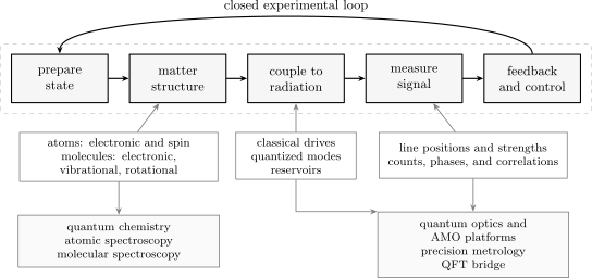
The common AMO workflow. Atomic and molecular structure determine available transitions; classical or quantized radiation couples them; measured spectra, counts, phases, and correlations feed back into preparation and control. Quantum chemistry, quantum optics, platforms, metrology, and the QFT bridge branch from different parts of the same loop.

Atomic, Molecular, and Optical Physics as Quantum Laboratories

An AMO experiment rarely observes a wavefunction directly. It prepares a state, applies fields, records outcomes, and compares the resulting statistics with a model. The physical system may be:

• an atom in a beam, vapor cell, trap, lattice, or cavity;
• a molecule with electronic, vibrational, rotational, nuclear-spin, and center-of-mass motion;
• one or more electromagnetic modes in coherent, thermal, number, squeezed, or more general states;
• a hybrid system in which matter and field excitations cannot be assigned independently;
• an ensemble whose collective signal is useful even when individual constituents are not resolved.

The laboratory description must say what is prepared and what is measured. “Hydrogen in a laser field” is not yet a reproducible problem. A specification may need the isotope, internal level, motional state, field polarization, propagation direction, pulse envelope, detuning, intensity convention, magnetic bias field, temperature, geometry, detection channel, and uncertainty model.

The operational state

If matter and selected radiation modes are both quantum, their joint state belongs to

$$\mathcal H_{\mathrm{tot}} = \mathcal H_{\mathrm m} \otimes \mathcal H_{\mathrm f}.$$

An initially uncorrelated preparation has the form

$$\rho_{\mathrm{tot}}(0) = \rho_{\mathrm m}(0) \otimes \rho_{\mathrm f}(0),$$

but an interaction generally creates matter–field correlations. When the field is treated as a prescribed classical drive, $\rho_{\mathrm f}$ is replaced by specified field amplitudes. When unobserved modes form a reservoir, they may be eliminated to obtain reduced dynamics for the retained system.

These are different models. A classical drive, a quantized cavity mode, and a traced-out vacuum reservoir should not be represented by the same symbol without explanation.

One Loop, Five Questions

Every chapter in this volume can be located by five questions.

Stage	Question	Typical mathematical object
Preparation	Which internal, motional, and field state is created?	state vector, density operator, ensemble, pulse sequence
Structure	Which energies, symmetries, and quantum numbers are available?	matter Hamiltonian, effective Hamiltonian, eigenstates
Coupling	Which field or environment connects the states?	interaction Hamiltonian, matrix elements, spectral density
Measurement	Which signal is recorded and with what response?	POVM, correlator, transition rate, line-shape model
Control	How are fields changed using the model or measurement record?	pulse envelope, feedback law, optimal-control functional

The output of one stage constrains the next. State preparation determines which initial populations and coherences are present. Internal structure determines resonance frequencies and selection rules. Coupling determines strengths and time scales. Measurement determines which information is accessible. Feedback changes the next preparation.

The Hierarchy of Resolved Scales

AMO physics often succeeds because different effects occupy separated energy or time scales. The hierarchy is not identical for every species, but a useful generic ladder is:

Scale or effect	Representative regime	Physical origin
Electronic structure	often electronvolts	Coulomb binding and electron correlation
Molecular vibration	often $10^{-2}$–$10^{-1}\,\mathrm{eV}$	nuclear motion in an electronic potential
Molecular rotation	often $10^{-5}$–$10^{-3}\,\mathrm{eV}$	rotational kinetic energy and moment of inertia
Fine structure	below gross electronic structure	relativistic kinematics, spin–orbit, and related terms
Hyperfine structure	usually below fine structure	nuclear moments coupled to electronic fields
Radiative shift	precision-dependent	coupling to quantized electromagnetic modes
Natural width	$\hbar/\tau$	finite lifetime $\tau$
Doppler or collisional width	apparatus-dependent	motion and environmental interactions
Driven shift	intensity-dependent	AC Stark, Autler–Townes, or dressing effects

The ranges are orientation scales, not reference data. Light molecules, floppy molecules, Rydberg states, highly charged ions, near-degenerate levels, and strongly driven systems can reorder the hierarchy.

Resolution chooses the effective theory

Suppose an experiment resolves gross, fine, and hyperfine structure. A useful effective Hamiltonian may be organized as

$$\begin{aligned} H_{\mathrm{eff}} ={}& H_{\mathrm{gross}} +\delta H_{\mathrm{fs}} +\delta H_{\mathrm{hfs}} \\ &+H_{\mathrm{ext}} +H_{\mathrm{drive}}. \end{aligned}$$

The experimental resolution determines which terms must be retained. If a correction is much smaller than both the target uncertainty and the relevant linewidth, it may be safely omitted for that observable. If two levels become nearly degenerate, even a nominally small term can dominate their mixing and must be treated nonperturbatively in the near-degenerate subspace.

Open-system effects are better written separately:

$$\frac{d\rho}{dt} = -\frac{i}{\hbar} \left[ H_{\mathrm{eff}}, \rho \right] +\mathcal D(\rho),$$

where $\mathcal D$ represents the stated reduced-dynamics model. A decay rate is not automatically a Hamiltonian correction, and a non-Hermitian effective Hamiltonian does not by itself specify the quantum jumps or unconditional density-operator evolution.

Three Central Objects

Matter Hamiltonians

The matter Hamiltonian determines the internal and motional structure that a field can address. Its detailed form depends on the problem:

• a hydrogenic Hamiltonian organizes one-electron Coulomb states;
• a central-field plus residual interaction organizes multi-electron atoms;
• an electron–nuclear Hamiltonian organizes molecular potential-energy surfaces;
• oscillator and rotor Hamiltonians organize low-lying molecular motion;
• spin, hyperfine, Zeeman, and Stark terms organize smaller splittings;
• effective few-level Hamiltonians organize controlled subspaces.

The canonical exact solutions remain in Wave Mechanics and Model Systems. This volume uses those solutions as components of physical models and specifies the corrections required by spectroscopy or control.

Radiation modes

Radiation can be represented at several levels.

Representation	State of the field	Appropriate questions
Prescribed classical field	amplitude, phase, polarization, envelope	coherent driving, weak spectroscopy, pulse control
Stochastic classical field	probability process or noise spectrum	technical noise, phase diffusion, inhomogeneous driving
Single quantized mode	number-state or density-operator description	cavity QED, photon exchange, number-dependent dynamics
Multimode quantum field	mode continuum and field correlations	spontaneous emission, photodetection, propagation
Reservoir model	spectral density and state	damping, pumping, dephasing, thermalization

A bright coherent field may admit an accurate semiclassical description for some observables. Photon antibunching, number-dependent splitting, entanglement with a cavity mode, and vacuum-induced effects require a quantum-field description.

Interaction Hamiltonians

The interaction selects which parts of matter and radiation can exchange energy, momentum, and angular momentum. In the electric-dipole regime,

$$H_{\mathrm{int}} \simeq -\mathbf d\cdot\mathbf E.$$

The matrix element

$$\langle f| \mathbf d\cdot\boldsymbol\epsilon |i\rangle$$

contains radial or vibrational structure, angular factors, and polarization geometry. Symmetry can force it to vanish. A vanishing electric-dipole element does not forbid all transitions; another multipole, magnetic coupling, collision, static-field mixing, or multiphoton process may remain.

The Wigner–Eckart Theorem owns the general angular decomposition. AMO applications supply the actual states, reduced matrix elements, field geometry, and measured signal.

Spectroscopy as a Measuring Language

Spectroscopy translates quantum structure into measured, frequency- or time-dependent data. Energy differences locate ideal resonances, but preparation, the interaction operator, dynamics, detection, and instrumental response determine what is actually recorded.

The Spectroscopy chapter overview owns the quantitative dictionary relating line positions, integrated strengths, widths, shapes, lifetimes, and time-domain coherences. The experimental-technique page owns instruments, calibration, resolution, and the historical evidence pipeline. Keeping those layers distinct prevents a fitted peak from being mistaken for a direct picture of an eigenvalue.

Lasers as Control Tools

A laser is not only a source for observing spectra. Its frequency, phase, polarization, intensity, spatial mode, and pulse envelope are control parameters in an effective Hamiltonian.

For an isolated resonant two-level system, define the pulse area

$$\Theta = \int_{t_i}^{t_f} \Omega(t)\,dt.$$

Under the ideal rotating-wave model and a fixed drive phase,

$$P_e = \sin^2 \left( \frac{\Theta}{2} \right).$$

A $\pi$ pulse ideally inverts the population, while a $\pi/2$ pulse creates an equal-amplitude superposition in the convention implied by the drive phase. This compact rule is useful because it converts a shaped field into a state-preparation target.

Its assumptions are substantial:

• a well-isolated two-level subspace;
• negligible detuning or a separately controlled detuning;
• a consistent Rabi-frequency convention;
• negligible spontaneous decay and dephasing during the pulse;
• negligible spatial inhomogeneity and motion-induced detuning;
• validity of the rotating-wave and dipole approximations.

When these assumptions fail, pulse area alone does not predict fidelity. Adiabatic passage, composite pulses, optimal control, and error-robust protocols address different failure modes.

Why AMO Platforms Matter

AMO platforms make parameters that are fixed in many natural systems experimentally adjustable.

Control knob	Hamiltonian or state effect	Typical platform
Laser frequency and phase	detuning, coherent rotation, interferometric phase	atoms, ions, molecules, cavities
Polarization	angular-momentum coupling and selection rules	spectroscopy and optical pumping
Magnetic field	Zeeman splitting, quantization axis, Feshbach tuning	traps and ultracold gases
Electric field	Stark shift, orientation, Rydberg interactions	molecules and Rydberg arrays
Trap frequency	motional spacing and wave-packet size	ions, neutral atoms, molecules
Lattice depth and geometry	tunneling, band structure, interaction ratios	optical lattices
Cavity geometry	mode spectrum and photonic density of states	cavity and circuit QED
Measurement record	conditional state and feedback signal	continuous monitoring and metrology

The platform page must also name what cannot be tuned freely: available species, level structure, selection rules, spontaneous decay, collisions, material loss, technical noise, and calibration limits.

Technology follows from metrology, not hype

Quantum technologies inherit their credibility from quantitative control and error accounting. A clock is useful because a transition can be prepared, interrogated, compared, and corrected with a traceable uncertainty budget. A qubit platform is useful when initialization, gates, readout, leakage, loss, and correlated noise are all characterized. A simulator is useful when its effective Hamiltonian and observables are calibrated against a reproducible model.

Connections Across the Subject

Destination	What leaves this overview	What the destination develops
Quantum chemistry	electron–nuclear Hamiltonians and scale separation	bonding, electronic structure, surfaces, reactions
Spectroscopy	transitions and line profiles	assignments, intensities, broadening, inference
Quantum optics	quantized modes and correlations	nonclassical states, detection, cavities, networks
Open systems	eliminated modes and noise	channels, master equations, trajectories, feedback
Many-body physics	tunable gases and lattices	collective phases, correlations, quasiparticles
Quantum information	controlled levels and photons	gates, algorithms, communication, error correction
Precision metrology	stable transitions and phase accumulation	clocks, standards, interferometry, systematic errors
QFT.org	quantized radiation and radiative corrections	field quantization, QED, renormalization, scattering

The same apparatus may support several destinations. An optical lattice can be an AMO trapping system, a realization of a many-body Hamiltonian, a quantum simulator, or a metrological sensor. Canonical ownership follows the question being answered.

Questions That Select the Next Chapter

• What are the intrinsic levels and quantum numbers? Continue to Atomic Physics, Multi-Electron Atoms, or Molecular Quantum Mechanics.
• What does a measured line mean? Continue to Spectroscopy.
• How does a drive produce coherent dynamics? Continue to Light–Matter Interaction.
• When must the field be quantized? Continue to Quantum Optics.
• How does gain produce sustained optical oscillation? Continue to Lasers.
• How are particles cooled, trapped, arranged, and read out? Continue to AMO Platforms and Quantum Control.
• How does a frequency become a standard or test? Continue to Precision Measurement and Metrology.
• How is the model solved and validated numerically? Continue to Computational AMO and Quantum Chemistry.
• Which claims are changing rapidly? Continue to Frontiers and Open Problems.

As those specialized pages are published, this overview will link to their canonical routes. Until then, the AMO Physics Roadmap and volume landing page provide live prerequisite handoffs.

Common Mistakes

Starting with a named effect instead of a model

“Zeeman effect,” “Rabi oscillation,” or “spontaneous emission” does not specify the retained levels, field geometry, coupling convention, or measurement. State the model before using the name.

Assuming the finest scale is always relevant

The required theory is selected by the target observable and uncertainty. Radiative or hyperfine corrections may be essential for a clock but irrelevant for a broad chemical trend. Conversely, a small term can dominate near a degeneracy.

Treating spectroscopy as an energy-only measurement

Line positions reveal energy differences. Intensities reveal operators, state preparation, polarization, and populations. Widths reveal dynamics and environment. Shapes reveal unresolved or interfering processes.

Treating classical and quantum light as rival descriptions

They answer different questions. A classical drive can accurately predict mean coherent dynamics in one regime, while photon statistics or matter–field entanglement require quantized modes.

Ignoring the detector

A calculated atomic correlator is not automatically the recorded count rate. Collection efficiency, mode matching, bandwidth, dead time, dark counts, filtering, calibration, and data processing can alter the signal.

Calling every controlled system a qubit

A two-level computational subspace may sit inside a larger Hilbert space. Leakage, spectator levels, motion, loss, and state-dependent detection remain physical even when the logical model is two dimensional.

Exercises

1. Audit a spectral claim

A paper says that a peak center is an excited-state energy, its height directly measures a transition matrix element, and its FWHM equals the inverse upper-state lifetime. Identify the missing qualifications.

Solution

The center normally constrains an energy difference, not one absolute energy, and may include recoil, field, collisional, radiative, and calibration shifts. Peak height also depends on population, degeneracy, polarization, linewidth, saturation, and instrument response; an integrated strength under stated conventions is usually the more stable comparison.

A lifetime can determine a Lorentzian contribution to the width only after ordinary versus angular frequency, HWHM versus FWHM, lower-state decay, and pure dephasing are specified. Doppler, collision, transit-time, power, inhomogeneous, unresolved-structure, source, and instrumental broadening must also be separated.

2. Decide whether two components are resolved

Two transitions are separated by angular frequency $\delta\omega$. Give a practical inequality involving their characteristic widths $\Gamma_1$, $\Gamma_2$, and instrumental resolution $\Gamma_{\mathrm{inst}}$ for treating them as clearly resolved. Explain why the criterion is not universal.

Solution

A conservative scale criterion is

$$\delta\omega \gg \max \left( \Gamma_1, \Gamma_2, \Gamma_{\mathrm{inst}} \right).$$

If the separation is comparable to the widths, the features overlap and should usually be fitted together. The exact resolution criterion depends on line shape, relative strength, noise, sampling, estimator, and whether prior information constrains the fit. There is no universal factor that replaces an explicit inference model.

3. Design ideal resonant pulses

What pulse areas prepare population inversion and an equal-population superposition in the ideal resonant two-level model? What additional control fixes the relative phase of the superposition?

Solution

A pulse area $\Theta=\pi$ gives ideal population inversion because $P_e=\sin^2(\pi/2)=1$. A pulse area $\Theta=\pi/2$ gives $P_e=1/2$.

The optical or microwave drive phase fixes the azimuthal direction of the rotation in the two-level Bloch sphere and therefore the relative phase of the prepared superposition. Pulse area alone fixes the rotation angle, not its full axis.

4. Choose a field description

For each observable, state whether a prescribed classical field can be sufficient or whether quantized modes are essential:

1. Mean Rabi oscillations driven by a bright stable laser.
2. Photon antibunching in resonance fluorescence.
3. Vacuum Rabi splitting in a single-emitter cavity.
4. AC Stark calibration far from resonance.

Solution

1. A prescribed classical drive can be sufficient for the mean coherent dynamics when laser noise and backaction are negligible.
2. Photon antibunching is a field-correlation measurement and requires quantized emitted radiation plus a detection model.
3. Vacuum Rabi splitting reflects coherent exchange with a quantized cavity mode and requires that mode explicitly.
4. A classical field can often describe an AC Stark calibration, provided spontaneous scattering and field fluctuations are either negligible or added consistently.

The choice is observable-dependent. The same laser may be classical in the system Hamiltonian while unobserved vacuum modes remain quantized in the decay model.

Cross-Links

• Atomic, Molecular, and Optical Physics
• Atomic Physics
• Multi-Electron Atoms
• Molecular Quantum Mechanics
• AMO Physics Roadmap
• Quantum Chemistry Roadmap
• Hydrogen Atom
• Two-Level Systems
• Wigner–Eckart Theorem
• Fermi’s Golden Rule
• Fock Space
• Open Quantum Systems

References

1. C. J. Foot, Atomic Physics, Oxford University Press, 2005.
2. B. H. Bransden and C. J. Joachain, Physics of Atoms and Molecules, 2nd ed., Pearson, 2003.
3. C. Cohen-Tannoudji, J. Dupont-Roc, and G. Grynberg, Atom–Photon Interactions: Basic Processes and Applications, Wiley, 1992.
4. P. W. Atkins and R. S. Friedman, Molecular Quantum Mechanics, 5th ed., Oxford University Press, 2011.
5. W. Demtröder, Laser Spectroscopy 1: Basic Principles, 5th ed., Springer, 2014.
6. M. O. Scully and M. S. Zubairy, Quantum Optics, Cambridge University Press, 1997.
7. D. A. Steck, Quantum and Atom Optics, revision 0.13.13, 2021.
8. H. J. Metcalf and P. van der Straten, Laser Cooling and Trapping, Springer, 1999.
9. H. J. Carmichael, Statistical Methods in Quantum Optics 1, Springer, 1999.
10. A. Kramida, Yu. Ralchenko, J. Reader, and the NIST ASD Team, NIST Atomic Spectra Database, National Institute of Standards and Technology, current evaluated release.