Instantons, Tunneling, and Nonperturbative Effects

A nonperturbative effect is an effect that is absent from every order of a specified perturbative expansion. The qualifier “specified” is essential. A term may be nonperturbative in $\hbar$, in a coupling $g$, or in an inverse occupation number, and those are different limiting statements.

Tunneling is the canonical quantum-mechanical example. In a semiclassical family, a transmission amplitude, bound-state splitting, or metastable decay rate may contain a factor such as

$$\exp\left( -\frac{S}{\hbar} \right).$$

No finite polynomial in $\hbar$ can produce this dependence. Yet the exponential alone is not a complete prediction: the action $S$, the relevant boundary conditions, the observable, the fluctuation prefactor, and the contributing saddle sectors must all be identified.

This chapter is the computational home for that organization. It does not duplicate the canonical derivations:

• Barrier Penetration and Tunneling owns the direct one-dimensional WKB transmission calculation.
• Euclidean and Imaginary-Time Path Integrals owns the Euclidean kernel, thermal trace, and operator meaning of imaginary-time evolution.
• Euclidean Time and Imaginary-Time Action owns the tunneling-oriented continuation, background subtraction, boundary variation, and fixed-energy exponent.
• Instantons in Quantum Mechanics Preview owns the path-integral derivation and explicit quartic instanton.
• Double-Well Tunneling owns the physical two-state splitting problem.
• Tunneling Splittings owns the quantitative conversion among the two-state coupling, Herring flux, WKB action, instanton sum, and measured spectral doublet.
• Instantons in Quantum Mechanics owns the Euclidean saddle method.
• Bounce Solutions owns the metastable boundary-value problem, round-trip action, and one-negative-mode diagnostic.
• False Vacuum Decay in Quantum Mechanics owns resonance widths, survival and nonescape probabilities, WKB escape rates, and the range of validity of exponential decay.
• Fluctuation Determinants Preview owns regulated determinant ratios, collective coordinates, and normalized prefactors.
• Asymptotic Series and Nonperturbative Corrections owns factorial growth, optimal truncation, beyond-all-orders scales, and the quartic-oscillator large-order lesson.
• Resurgence Preview owns the advanced relation between perturbative and nonperturbative sectors.

The purpose of this overview is to define the language, separate the principal observables, and show where each calculation belongs.

What Nonperturbative Means

Let $\epsilon$ be a dimensionless small parameter. An ordinary perturbative sector has the formal structure

$$Q_{\mathrm{pert}}(\epsilon) \sim \sum_{n=0}^{\infty} a_n\epsilon^n, \qquad \epsilon\to0^+.$$

Now take $A\gt0$. For every fixed nonnegative integer $N$,

$$\lim_{\epsilon\to0^+} \frac{e^{-A/\epsilon}}{\epsilon^N} = 0.$$

The exponential is therefore beyond all algebraic orders in $\epsilon$: it is smaller than every power as the limit is approached. A contribution

$$Q_{\mathrm{np}}(\epsilon) = C\epsilon^\beta e^{-A/\epsilon} \left[ 1+O(\epsilon) \right]$$

cannot be recovered from any finite truncation of the power series.

This definition has several consequences.

1. Nonperturbative does not mean large. The effect is often exponentially small in the regime where it is most cleanly calculated.
2. Nonperturbative does not mean strong coupling. Weak-coupling gauge theory can contain terms proportional to $e^{-8\pi^2/g^2}$.
3. Nonperturbative does not mean exact. An instanton calculation is itself a semiclassical asymptotic approximation.
4. Nonperturbative does not identify a mechanism. Instantons are one source; complex saddles, boundary effects, topology, and other singular structures can also contribute.
5. The expansion parameter must be named. Calling a result “nonperturbative” without saying “in what” is incomplete.

Flat functions and local information

Extend

$$f(\epsilon) = e^{-A/\epsilon}$$

for $\epsilon\gt0$ by setting $f(0)=0$. Every right derivative at $\epsilon=0$ vanishes. Its Taylor series at the origin is therefore identically zero even though $f(\epsilon)$ is nonzero for every positive $\epsilon$.

This is the simplest model of why local expansion data can miss global saddle information. The missing contribution is not an unusually high perturbative order. It belongs to a different asymptotic sector.

Asymptotic Series and Exponential Sectors

Perturbative series in quantum mechanics are often asymptotic rather than convergent. For fixed truncation order $N$,

$$Q(\epsilon) = \sum_{n=0}^{N-1} a_n\epsilon^n + R_N(\epsilon),$$

where the first omitted term may initially estimate the remainder. If the coefficients eventually grow factorially, adding terms past the optimal order makes the approximation worse.

An exponentially improved expansion can have the schematic form

$$\begin{aligned} Q(\epsilon) &\sim \sum_{n\ge0} a_{0,n}\epsilon^n \\ &\quad + \sum_{k\ge1} \sigma^k e^{-kA/\epsilon} \epsilon^{\beta_k} \sum_{n\ge0} a_{k,n}\epsilon^n. \end{aligned}$$

The $k=0$ sector is perturbative around a reference saddle. The sectors $k\ge1$ can represent one instanton, several instantons, or other saddles. The coefficient $\sigma$ summarizes boundary conditions or a contour prescription; it is not an arbitrary correction inserted after the fact.

This schematic form should not be applied mechanically. The relevant actions can be complex, several inequivalent saddles can compete, logarithms can appear, and the sector structure can change across Stokes lines. The cautious conclusion is that a local power series and a global saddle analysis are complementary, not rival descriptions.

Three Tunneling Observables

The word “tunneling” covers several observables. Their exponents are related, but they are not interchangeable.

For a one-dimensional forbidden interval $x_1\lt x\lt x_2$, define the one-way under-barrier action

$$K(E) = \int_{x_1}^{x_2} \sqrt{2m[V(x)-E]}\,dx.$$

Problem	Boundary condition and observable	Leading exponential structure
Open-barrier scattering	Incoming wave on one side; transmitted flux on the other	$t(E)\sim e^{-K(E)/\hbar}$ and $T(E)\sim e^{-2K(E)/\hbar}$
Symmetric bound double well	Normalizable parity eigenstates; energy splitting	$\Delta E\sim A_{\mathrm{split}}e^{-K(E_{\mathrm{loc}})/\hbar}$
Metastable well	Outgoing resonance boundary condition; survival or decay rate	$\gamma\sim A_{\mathrm{decay}}e^{-B/\hbar}$

The transmission amplitude $t$, probability $T$, splitting $\Delta E$, and decay rate $\gamma$ have different units and normalizations. In a one-dimensional metastable problem, the bounce action $B$ often corresponds at leading order to an outward-and-return Euclidean path and is related to twice a one-way forbidden action. That factor must be derived from the boundary-value problem, not guessed from a neighboring formula.

This distinction also explains why “the tunneling probability” is not a universal object. A stationary bound state has no incident flux, and a metastable resonance is not an exact normalizable eigenstate. The physical question comes before the exponent.

Why Euclidean Time Helps

A real-time path integral carries the oscillatory weight

$$\exp\left( \frac{i}{\hbar}S[x] \right).$$

Under a justified contour rotation $t=-i\tau$, the imaginary-time kernel is

$$K_E(x_f,T;x_i,0) = \langle x_f\vert e^{-\hat H T/\hbar} \vert x_i\rangle$$

and has the formal representation

$$K_E = \int\mathcal D x\, \exp\left[ -\frac{1}{\hbar}S_E[x] \right],$$

with

$$S_E[x] = \int_0^T d\tau \left[ \frac{m}{2} \left( \frac{dx}{d\tau} \right)^2 + V(x) \right].$$

The positive kinetic term and damping weight turn certain tunneling questions into saddle-point problems resembling statistical mechanics. Stationarity gives

$$m\frac{d^2x}{d\tau^2} = V'(x),$$

which is equivalent to ordinary classical motion in the inverted potential $-V(x)$ as a solution-finding analogy.

That analogy must not be literalized. An instanton is not a hidden real-time trajectory of a particle moving through the barrier. It is a stationary configuration used to evaluate a quantum amplitude after analytic continuation.

Ground-state projection

If

$$\vert\Psi\rangle = \sum_n c_n\vert n\rangle$$

and $c_0\ne0$, then

$$\vert\Psi(T)\rangle \equiv e^{-\hat H T/\hbar}\vert\Psi\rangle.$$

Factoring out the slowest decaying exponential gives

$$\begin{aligned} \vert\Psi(T)\rangle &= e^{-E_0T/\hbar} \Bigg[ c_0\vert0\rangle \\ &\quad+ \sum_{n\gt0}c_n e^{-(E_n-E_0)T/\hbar} \vert n\rangle \Bigg]. \end{aligned}$$

Large Euclidean time suppresses excited states relative to the ground state. In a double well, the tiny difference between the two lowest exponents encodes the tunneling splitting. In a metastable problem, analytic continuation of the Euclidean saddle calculation instead reveals an imaginary part associated with decay.

Wick rotation can fail or require refinement when singularities obstruct the contour, when the Hamiltonian is not bounded below, or when real-time boundary conditions are not obtained by naive continuation. The Euclidean formulation is a method with assumptions, not a universal deletion of the factor $i$.

The Euclidean Saddle Dictionary

Different boundary conditions select different stationary configurations.

Configuration	Euclidean boundary data	Physical role	Characteristic fluctuation feature
Vacuum saddle	Remains near one minimum	Perturbative reference sector	Positive spectrum after exact symmetries are handled
Instanton	Connects distinct degenerate minima or sectors	Tunneling amplitude and level splitting	Translational zero mode
Anti-instanton	Reverse connection	Oppositely oriented tunneling event	Translational zero mode
Multi-instanton configuration	Several well-separated transitions	Repeated events and sector sums	Collective coordinates and interactions
Bounce	Leaves and returns to a metastable minimum	Imaginary part and decay rate	One negative mode plus translation zero mode
Complex saddle	Complexified coordinates or contour	Oscillatory or otherwise inaccessible sectors	Contour- and Stokes-dependent

The number of zero and negative modes is not decorative bookkeeping. It helps identify what the saddle computes. A translation zero mode means the event center is arbitrary and must be integrated as a collective coordinate. A negative mode means the stationary configuration is not a local minimum of $S_E$; for a bounce, the corresponding contour deformation is tied to the imaginary part of a metastable energy.

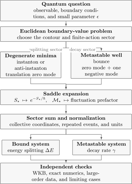
The observable fixes the boundary-value problem before the saddle is chosen. Degenerate minima lead to instantons and splittings; a metastable well leads to a bounce and a decay rate. In either branch, the Euclidean action gives the exponent, fluctuations give the prefactor, and sector sums plus independent checks turn a saddle weight into a physical prediction.

Instantons and Bounces

Instantons between degenerate minima

For a double well with degenerate minima shifted to $V=0$, finite action requires

$$x(\tau)\to x_\pm, \qquad \frac{dx}{d\tau}\to0, \qquad \tau\to\pm\infty.$$

The conserved Euclidean energy is then zero:

$$\frac{m}{2} \left( \frac{dx}{d\tau} \right)^2 - V(x) = 0.$$

For a monotone instanton,

$$S_I = \int_{x_-}^{x_+} \sqrt{2mV(x)}\,dx.$$

This is the same geometric action that controls the leading WKB barrier amplitude at zero reference energy. Instantons in Quantum Mechanics Preview derives the result and solves the quartic double well explicitly; Double-Well Tunneling connects it to the parity splitting.

Bounces from a metastable well

A metastable state is localized near a local minimum but can escape through a barrier. Its resonance energy can be written

$$E_{\mathrm{res}} = E_F - \frac{i\hbar\gamma}{2},$$

so a survival probability behaves as

$$P_{\mathrm{surv}}(t) \sim e^{-\gamma t}$$

over the exponential-decay regime.

The corresponding Euclidean bounce begins near the false minimum, reaches a turning point beyond the barrier, and returns. Its semiclassical contribution has the structure

$$\gamma \sim A_{\mathrm{bounce}} e^{-B/\hbar} \left[ 1+O(\epsilon) \right].$$

The bounce is not merely an instanton whose endpoints happen to coincide. Its boundary conditions, one-negative-mode structure, and physical interpretation differ. Bounce Solutions derives the classical profile, round-trip action, and mode diagnostic. The simple exponential-decay regime can also fail at very short and very long times, so $\gamma$ is an intermediate-time resonance property rather than an exact all-time law.

Exponent, Prefactor, and Sector Sum

A reliable saddle calculation has three levels.

1. The exponent

Solve the Euclidean boundary-value problem and evaluate

$$S_\star = S_E[x_\star].$$

This gives $e^{-S_\star/\hbar}$. The exponent usually controls the dominant parameter dependence when $S_\star/\hbar\gg1$.

2. The prefactor

Write

$$x(\tau) = x_\star(\tau) + \eta(\tau).$$

The quadratic fluctuation operator is

$$\mathcal M_\star = - m\frac{d^2}{d\tau^2} + V''(x_\star).$$

Gaussian integration produces a regulated determinant ratio. Exact zero modes are removed from the determinant and replaced by collective-coordinate integrals; negative modes require a contour prescription. Units, state normalization, and boundary conditions all enter the prefactor.

3. The sector sum

A physical kernel can require the trivial saddle, instantons, anti-instantons, and repeated events. In a dilute regime, widely separated events can be summed combinatorially. Beyond that regime, saddle interactions, quasi-zero modes, complex saddles, and Stokes phenomena can matter.

Stopping after the exponent is legitimate only if the claim is explicitly limited to logarithmic or leading-exponential accuracy. If $Q_0$ is a reference scale without exponential dependence and $\epsilon_\star=\hbar/S_\star$, that claim can be written

$$\begin{gathered} \epsilon_\star\to0^+, \\ -\epsilon_\star \log\left| \frac{Q}{Q_0} \right| \longrightarrow 1. \end{gathered}$$

It is not enough for a normalized rate, a precision splitting, or a comparison of two saddles with nearly equal actions.

Relation to WKB and Perturbation Theory

WKB and instanton methods often reproduce the same one-dimensional tunneling action because both are semiclassical descriptions of the same Schrödinger problem.

Method	Natural representation	Main strength	Typical limitation
Forbidden-region WKB	Stationary Schrödinger equation	Direct transmission, connection formulas, energy-dependent barriers	Global multi-saddle organization can be awkward
Instanton calculus	Euclidean path integral	Global saddle sectors, collective coordinates, multidimensional and field-theory generalization	Contours, determinants, and mode treatment are demanding
Local perturbation theory	Expansion around one minimum	Accurate algebraic corrections within one well	Misses inter-well splitting at every finite order
Exact diagonalization	Basis or spatial grid	Benchmark spectra and wavefunctions	Exponentially small splittings demand precision and large domains
Resurgent analysis	Large-order and Borel data	Connects local series to other saddle sectors in favorable models	Requires analytic continuation and model-dependent saddle information

The correct conclusion is not that perturbation theory “fails” whenever an instanton exists. Perturbation theory computes fluctuations around a chosen saddle; instantons add sectors associated with other saddles. A complete semiclassical answer can require both:

$$\begin{gathered} \text{local fluctuation series} \\ {}+\ \text{nontrivial saddle sectors}. \end{gathered}$$

For the double well, the perturbative expansion around either minimum can accurately describe the mean energy of a nearly degenerate pair, while the instanton sector supplies the exponentially small difference between the two parity levels.

Method Roadmap

Question	Canonical page
How does a symmetric double well produce localized states and an even–odd splitting?	Double-Well Tunneling
How are two-state, Herring, WKB, and instanton splitting estimates matched?	Tunneling Splittings
How are the Euclidean action, boundary data, and fixed-energy tunneling exponent obtained?	Euclidean Time and Imaginary-Time Action
How is a finite-action Euclidean solution constructed and evaluated?	Instantons in Quantum Mechanics
How is a metastable bounce constructed and how is its decay exponent evaluated?	Bounce Solutions
How does a bounce exponent become a resonance lifetime and when is decay exponential?	False Vacuum Decay in Quantum Mechanics
Where do determinant prefactors, zero modes, and negative modes enter?	Fluctuation Determinants Preview
Why can a useful perturbation series diverge, and where should it be truncated?	Asymptotic Series and Nonperturbative Corrections
How can perturbative large-order behavior communicate with instanton sectors?	Resurgence Preview
Which parts of quantum-mechanical instanton logic survive in field theory?	Bridge to QFT Instantons
How is the same barrier treated directly in wave mechanics?	Barrier Penetration and Tunneling
What does the imaginary-time kernel mean as an operator?	Euclidean and Imaginary-Time Path Integrals

Reliability Checklist

Before trusting a nonperturbative semiclassical result, state:

1. Expansion parameter: Is the small parameter $\hbar/S_\star$, $g$, $g^2$, or something else?
2. Observable: Is the result an amplitude, probability, splitting, energy width, or decay rate?
3. Boundary conditions: Which initial, final, normalizability, periodicity, or outgoing conditions define the problem?
4. Contour: Why is the Euclidean or complexified integration cycle appropriate?
5. Saddle inventory: Which trivial, instanton, anti-instanton, bounce, or complex saddles contribute?
6. Action hierarchy: Are competing actions parametrically separated?
7. Mode spectrum: How are zero modes, negative modes, and exact symmetries treated?
8. Prefactor units: Does the prefactor have the dimensions required by the observable?
9. Sector approximation: Is a one-saddle or dilute-gas approximation justified?
10. Independent check: Does WKB, exact diagonalization, large-order data, or direct numerical evolution confirm the result?

Action accuracy is especially unforgiving. If

$$Q \propto e^{-S/\hbar},$$

then an action error $\delta S$ changes the leading answer by

$$\frac{Q(S+\delta S)}{Q(S)} = e^{-\delta S/\hbar}.$$

A small relative error in a large action need not be a small error in the exponential. Prefactor-level accuracy requires controlling $\delta S$ on the scale of $\hbar$, not merely on the scale of $S$.

Standard Results and Active Boundaries

The following claims are standard in their established regimes:

• tunneling effects can be beyond all orders in a local power expansion;
• finite-action Euclidean saddles determine leading semiclassical exponents;
• double-well instantons reproduce the leading under-barrier action;
• translational invariance produces a collective-coordinate zero mode;
• a metastable bounce has a negative mode tied to decay;
• fluctuation determinants supply prefactors;
• multi-instanton sectors are needed for complete low-energy kernels in the dilute regime.

More advanced questions remain model-dependent or active:

• whether a proposed set of real and complex saddles is complete;
• how Stokes phenomena select contributing thimbles;
• how nonperturbative sectors are reconstructed from limited perturbative data;
• how resurgence extends across broad classes of quantum field theories;
• how instantons compete with renormalons, strong coupling, or other mechanisms.

The Resurgence Preview marks that boundary explicitly. The Bridge to QFT Instantons explains why the saddle logic survives in field theory while gauge fixing, topology, fermion zero modes, and renormalization require new machinery.

Common Mistakes

• Calling a result nonperturbative without naming the expansion parameter.
• Treating “nonperturbative” as a synonym for exact, numerical, or strong coupling.
• Assuming a divergent perturbative series contains no useful information.
• Using one formula for transmission, splitting, and decay without rederiving the boundary conditions.
• Squaring an amplitude exponent twice or not at all.
• Treating the inverted-potential analogy as a literal real-time trajectory.
• Calling every Euclidean solution an instanton without checking finite action and asymptotic data.
• Confusing a double-well instanton zero mode with a bounce negative mode.
• Quoting $e^{-S/\hbar}$ as a complete rate while omitting the prefactor and its units.
• Ignoring anti-instantons or repeated events when the kernel requires a sector sum.
• Assuming Wick rotation is valid without checking singularities and contours.
• Claiming that instantons capture every nonperturbative effect.

Exercises

1. Prove exponential smallness beyond all powers

Let $A\gt0$ and $N$ be a fixed nonnegative integer. Prove that

$$\lim_{\epsilon\to0^+} \frac{e^{-A/\epsilon}}{\epsilon^N} = 0.$$

Solution

Set $y=A/\epsilon$. Then $\epsilon\to0^+$ corresponds to $y\to\infty$, and

$$\frac{e^{-A/\epsilon}}{\epsilon^N} = \frac{y^N}{A^N}e^{-y}.$$

The exponential dominates every fixed power. For example, repeated use of l’Hôpital’s rule gives

$$\lim_{y\to\infty} \frac{y^N}{e^y} = \lim_{y\to\infty} \frac{N!}{e^y} = 0.$$

Multiplication by the fixed factor $A^{-N}$ does not change the limit. Thus $e^{-A/\epsilon}=o(\epsilon^N)$ for every fixed $N$.

2. Distinguish amplitude and probability exponents

Suppose a WKB transmission amplitude has leading form

$$t(E) \sim C(E)e^{-K(E)/\hbar}.$$

Find the leading transmission probability and explain why the same factor of two should not automatically be inserted into a bound-state splitting.

Solution

The transmission probability is a flux ratio. When incident and transmitted velocity factors have been included in $C$, its leading exponential is

$$T(E) \sim \lvert C(E)\rvert^2 e^{-2K(E)/\hbar}.$$

The exponent doubles because a probability is quadratic in the amplitude.

A double-well splitting is itself linear in the off-diagonal tunneling matrix element:

$$\Delta E = 2\lvert H_{LR}\rvert.$$

Since $H_{LR}$ is amplitude-level, its leading exponential is ordinarily $e^{-K/\hbar}$ rather than $e^{-2K/\hbar}$. The observable and its normalization determine whether an amplitude is squared.

3. Show imaginary-time ground-state projection

Let $\hat H\vert n\rangle=E_n\vert n\rangle$, with $E_0\lt E_1\le E_2\le\cdots$, and let $c_0\ne0$ in

$$\vert\Psi\rangle = \sum_n c_n\vert n\rangle.$$

Show that the normalized state proportional to $e^{-\hat H T/\hbar}\vert\Psi\rangle$ approaches $\vert0\rangle$ as $T\to\infty$.

Solution

Spectral decomposition gives

$$\vert\Psi(T)\rangle \equiv e^{-\hat H T/\hbar}\vert\Psi\rangle.$$

Therefore

$$\begin{aligned} \vert\Psi(T)\rangle &= \sum_n c_ne^{-E_nT/\hbar}\vert n\rangle \\ &= e^{-E_0T/\hbar} \Bigg[ c_0\vert0\rangle \\ &\quad+ \sum_{n\gt0}c_n e^{-(E_n-E_0)T/\hbar} \vert n\rangle \Bigg]. \end{aligned}$$

Every excited-state coefficient relative to the ground-state coefficient contains

$$e^{-(E_n-E_0)T/\hbar} \longrightarrow 0.$$

After normalization, only the component parallel to $\vert0\rangle$ remains. If the ground state is degenerate, the limit projects onto the component in the ground-state subspace rather than onto one unique vector.

4. Match the instanton and WKB actions

For degenerate minima with $V(x_\pm)=0$, suppose an instanton has zero Euclidean energy:

$$\frac{m}{2} \left( \frac{dx}{d\tau} \right)^2 = V(x).$$

Show that its Euclidean action is

$$S_I = \int_{x_-}^{x_+} \sqrt{2mV(x)}\,dx,$$

and identify the corresponding WKB quantity.

Solution

Along the zero-energy solution, the kinetic and potential terms are equal. Hence

$$\begin{aligned} S_I &= \int d\tau \left[ \frac{m}{2}(x')^2+V(x) \right] \\ &= \int d\tau\,2V(x). \end{aligned}$$

For a monotone instanton,

$$x' = \sqrt{\frac{2V(x)}{m}}, \qquad d\tau = dx\sqrt{\frac{m}{2V(x)}}.$$

Therefore

$$S_I = \int_{x_-}^{x_+} \sqrt{2mV(x)}\,dx.$$

This is the one-way WKB forbidden action

$$K(E) = \int \sqrt{2m[V(x)-E]}\,dx$$

evaluated here at the energy convention $E=0$ of the degenerate minima.

5. Classify the saddle from its modes

Two Euclidean saddles both have a translation zero mode. Saddle A connects two degenerate minima. Saddle B starts and ends at the same metastable minimum and has one additional negative eigenvalue. Classify the saddles and state their usual physical roles.

Solution

Saddle A is an instanton. It connects distinct degenerate minima or sectors and contributes to a tunneling amplitude and, after the appropriate sector sum, to a bound-state splitting.

Saddle B is a bounce. It leaves and returns to a false minimum. Its translation zero mode locates the event in Euclidean time, while the additional negative mode signals the contour direction responsible for the imaginary part of the metastable energy. That imaginary part determines a decay rate.

6. Quantify sensitivity to action error

A leading prediction is $Q\propto e^{-S/\hbar}$ with $S/\hbar=30$. If an approximate saddle action is high by one percent, by what factor is the predicted $Q$ changed? What relative action accuracy keeps the exponential error below ten percent?

Solution

A one-percent error gives

$$\frac{\delta S}{\hbar} = 0.01\frac{S}{\hbar} = 0.30.$$

Because the action is overestimated,

$$\frac{Q_{\mathrm{approx}}}{Q_{\mathrm{true}}} = e^{-0.30} \simeq 0.741.$$

The result is about $26$ percent low even though the action error is only one percent.

To keep the multiplicative error below ten percent, require

$$e^{\lvert\delta S\rvert/\hbar} \lt 1.10.$$

Thus

$$\frac{\lvert\delta S\rvert}{\hbar} \lt \log(1.10) \simeq 0.0953.$$

Since $S/\hbar=30$,

$$\frac{\lvert\delta S\rvert}{S} \lt \frac{0.0953}{30} \simeq 3.18\times10^{-3}.$$

The action must therefore be accurate to about $0.32$ percent for this criterion.

References

1. S. Coleman, Aspects of Symmetry (Cambridge University Press, 1985), especially “The Uses of Instantons” and “The Fate of the False Vacuum.” The classic pedagogical treatment of instantons, bounces, collective coordinates, and dilute gases.
2. R. Rajaraman, Solitons and Instantons (North-Holland, 1982). Detailed treatment of finite-action solutions and their fluctuation spectra.
3. J. Zinn-Justin, Path Integrals in Quantum Mechanics (Oxford University Press, 2005). Systematic account of Euclidean path integrals, semiclassical expansions, instantons, and large-order behavior.
4. H. Kleinert, Path Integrals in Quantum Mechanics, Statistics, Polymer Physics, and Financial Markets, 5th ed. (World Scientific, 2009). Broad reference on path-integral and semiclassical techniques.
5. A. Garg, “Tunnel splittings for one-dimensional potential wells revisited”, American Journal of Physics 68, 430–437 (2000). Careful comparison of WKB and instanton splitting formulas and prefactors.
6. C. M. Bender and T. T. Wu, “Anharmonic Oscillator”, Physical Review 184, 1231–1260 (1969). Foundational analysis of divergent perturbation theory and large-order behavior.
7. J. Zinn-Justin and U. D. Jentschura, “Multi-instantons and exact results I: conjectures, WKB expansions, and instanton interactions”, Annals of Physics 313, 197–267 (2004). Detailed relation among WKB, instanton sectors, and generalized expansions in quantum mechanics.
8. S. Coleman, “Fate of the false vacuum: Semiclassical theory”, Physical Review D 15, 2929–2936 (1977). Canonical derivation of the bounce exponent in field theory.
9. C. G. Callan Jr. and S. Coleman, “Fate of the false vacuum. II. First quantum corrections”, Physical Review D 16, 1762–1768 (1977). Fluctuation prefactor and decay-rate framework.
10. G. V. Dunne and M. Ünsal, “Uniform WKB, multi-instantons, and resurgent trans-series”, Physical Review D 89, 105009 (2014). Modern connection among uniform WKB, instantons, and resurgence in quantum-mechanical models.