AMO Platforms and Quantum Control

An AMO platform is an experimentally controlled quantum system built from atomic, molecular, optical, or closely analogous degrees of freedom. A platform is more than a species, trap, or qubit. It is the complete, calibrated chain that prepares a state, realizes a Hamiltonian or quantum channel, measures an outcome, and assigns an uncertainty to the inference.

That systems-engineering definition matters. An atom can possess an exceptionally narrow transition and still make a poor sensor if the atoms cannot be loaded reproducibly. A qubit can have a long coherence time and still make a poor processor if its gates leak outside the computational subspace. A trap can confine particles for minutes and still be unsuitable for many-body physics if its temperature, density, or interaction parameters are not known. The useful object is therefore not isolated hardware but a closed experimental control cycle.

AMO experiments are unusually clean because their microscopic constituents, couplings, and measurement channels can often be identified one by one. They are not clean because noise has disappeared. Laser phase noise, magnetic-field drift, blackbody radiation, photon scattering, motional heating, collisions, imperfect vacuum, detector errors, and calibration drift remain part of the physical model.

Canonical Scope

This page is the conceptual and quantitative map of AMO platforms. It owns:

1. the distinction between a physical platform, a chosen model, and a qubit;
2. the preparation–control–evolution–measurement–feedback cycle;
3. a common open-system control model for comparing otherwise different hardware;
4. the main trade-offs among neutral atoms, trapped ions, molecules, atom–cavity systems, photons, and superconducting circuits;
5. the roles of AMO platforms in quantum simulation, quantum information, and precision measurement;
6. the minimum validation and error-budget questions that make a platform claim scientifically meaningful.

Detailed mechanisms have separate canonical homes. The present overview does not rederive Doppler forces, polarization-gradient cooling, optical trap depths, Paul-trap stability, sideband gates, Rydberg blockade, Hubbard-model reductions, or interferometer scale factors. Those derivations belong to the dedicated pages in this chapter and to the relevant formalism volumes.

Rabi Oscillations owns coherent two-level dynamics. AC Stark Shift owns light shifts and the basic dispersive interaction behind optical trapping. Cavity QED owns the single-emitter cavity parameters and strong-coupling regimes. Quantum Control and Feedback owns general control, estimation, and feedback theory. POVMs owns generalized measurement statistics. Bose–Einstein Condensation and the Hubbard Model own their general many-body theories.

A Common Mathematical Model

Many platforms can be described, over a declared operating regime, by

$$H(t;\boldsymbol{\theta}) = H_0(\boldsymbol{\theta}) + \sum_k u_k(t)H_k,$$

where:

• $H_0$ contains uncontrolled or slowly tuned system parameters $\boldsymbol{\theta}$;
• $u_k(t)$ are classical control waveforms such as laser amplitudes, phases, frequencies, magnetic fields, electrode voltages, or microwave envelopes;
• $H_k$ are the operators through which those controls act.

For an open system, a common Markovian working model is

$$\dot{\rho} = -\frac{i}{\hbar}[H(t),\rho] + \sum_\mu \gamma_\mu \mathcal D[L_\mu]\rho,$$

with

$$\mathcal D[L]\rho = L\rho L^\dagger -\frac{1}{2} \left\{ L^\dagger L,\rho \right\}.$$

This equation is not a declaration that every laboratory environment is Markovian. It is a compact engineering model whose validity must be tested over the bandwidth and duration of the experiment. Colored laser noise, quasistatic field drift, trap-loss events, collision histories, and feedback latency can require stochastic Hamiltonians, non-Markovian models, or explicit classical state variables.

A measurement with outcome $y$ is represented at the probability level by positive operators $E_y$:

$$p(y|\rho,\boldsymbol{\theta}) = \operatorname{Tr}(E_y\rho), \qquad \sum_y E_y=I.$$

The physical state update requires a quantum instrument, not only the POVM. In many AMO experiments, however, the immediate inference problem is already substantial: $E_y$ must include finite photon collection, dark counts, thresholding, state leakage, atom loss, optical pumping during detection, and spatially varying response.

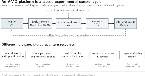
AMO hardware differs greatly, but the logical experiment is shared. A state $\rho_0$ is prepared, controls $u_k(t)$ shape the dynamics, an evolution $\mathcal E_t$ acts in the presence of noise, and a calibrated measurement $\{E_y\}$ produces data. Inference and feedback close the loop. Isolation is useful only when every arrow is characterized.

The Platform Is the Whole Cycle

The cycle in the figure separates five questions that are too often folded into the single word control.

Preparation

What density operator enters the experiment?

Preparation may include:

• slowing and capturing a thermal beam;
• laser cooling or sympathetic cooling;
• evaporative cooling;
• optical pumping into a Zeeman or hyperfine state;
• resolved-sideband cooling of a motional mode;
• deterministic rearrangement of a neutral-atom array;
• heralding a photon or cavity state;
• initializing a superconducting circuit by relaxation, measurement, or active reset.

A quoted temperature does not completely specify the state. One may also need the particle-number distribution, internal-state purity, motional-mode occupations, spatial correlations, condensate fraction, or residual entanglement with preparation apparatus.

Control

Which terms in $H(t)$ are independently programmable, with what bandwidth, dynamic range, spatial resolution, and calibration uncertainty?

A nominal Rabi frequency $\Omega$ is not yet a control specification. Its amplitude and phase noise, detuning, spatial profile, polarization, turn-on transient, off-resonant couplings, and correlations with other controls can all matter. In an array, the response is generally $\Omega_j(t)$ rather than one global number.

Evolution

Which degrees of freedom are retained in the model, and which are treated as an environment?

Examples include:

• an internal clock doublet coupled to external motion;
• spins coupled through phonon modes in an ion chain;
• atoms tunneling and interacting in optical-lattice bands;
• Rydberg states coupled by van der Waals or resonant dipole interactions;
• a two-level emitter coupled to a lossy cavity mode;
• a superconducting artificial atom coupled to resonators and transmission lines.

Model reduction is part of platform design. It must be supported by scale separation, not merely by the desire for a simple Hamiltonian.

Measurement

Which observable is inferred, from which raw detector record?

State-dependent fluorescence, absorption images, phase-contrast images, ionization, cavity transmission, homodyne current, dispersive microwave readout, and time-tagged photon counts implement different quantum instruments. The final binary label in a data file may conceal a continuous photon record and a nontrivial classifier.

Inference and feedback

How are uncertain parameters estimated and controls updated?

Feedback occurs on several time scales:

• fast analog or digital feedback within one experimental shot;
• adaptive selection of a later pulse based on an earlier measurement;
• shot-to-shot correction of laser, magnetic-field, or trap drift;
• periodic recalibration of amplitudes, detunings, imaging thresholds, and transfer functions;
• long-term maintenance of vacuum, alignment, and reference standards.

The Laser Stabilization page gives the canonical frequency-domain treatment of a representative laboratory feedback loop.

Why AMO Systems Can Be Clean

Several favorable features occur together.

Reproducible microscopic constituents

Two atoms of the same isotope in the same internal state are, within the Standard Model and the declared environment, identical quantum systems. Their transition frequencies and matrix elements do not vary because of fabrication disorder. This does not eliminate environmental inhomogeneity, collisional shifts, or differential light shifts, but it sharply separates the constituent from its apparatus.

Sparse, addressable spectra

Atomic and molecular levels provide resolved transitions with selection rules. Lasers and microwave sources can address particular couplings in frequency, polarization, space, and time. The same spectral structure can also be a liability: molecules have many rotational and vibrational leakage channels, while multilevel atoms can suffer unwanted Raman processes and light shifts.

Isolation and long coherence

Ultrahigh vacuum suppresses collisions. Trapping separates particles from material walls. Hyperfine, Zeeman-insensitive, clock, and metastable states can be weakly coupled to environmental noise. Cryogenic electromagnetic modes can have long lifetimes.

Isolation is never absolute. It shifts the dominant error mechanisms toward effects that would be negligible in ordinary conditions: blackbody shifts, stray dc fields, polarization ellipticity, electric-field noise near surfaces, phase noise on radio-frequency sources, and rare background-gas collisions.

Tunable energy and length scales

Optical wavelengths set micron and submicron structure. Trap frequencies, detunings, Rabi frequencies, scattering lengths, lattice depths, and interaction geometries can be varied over useful ranges. Feshbach resonances, Rydberg excitation, cavity mediation, and microwave dressing offer qualitatively different interaction mechanisms.

Tunability does not mean independent tunability. Increasing optical power may deepen a trap while increasing scattering and differential Stark shifts. Increasing confinement can strengthen interactions while increasing sensitivity to heating or anharmonicity. Every tuning knob belongs in a coupled error budget.

Efficient, state-selective detection

Cycling transitions can scatter many photons conditional on internal state. Quantum gas microscopes can resolve individual lattice sites. Cavity enhancement can make weak dispersive signals detectable. Trapped-ion fluorescence can approach near-projective internal-state readout.

High raw contrast does not remove the need to distinguish preparation, measurement, and loss errors.

A Scale Hierarchy for Control

No single figure of merit ranks every AMO platform, but a useful experiment usually establishes several inequalities.

For a coherent operation at scale $\Omega$,

$$\Omega \gg \Gamma_{\mathrm{decoh}}, \Gamma_{\mathrm{loss}}, \Gamma_{\mathrm{heat}},$$

where each rate must be interpreted for the relevant state and mode. The rough number of coherent radians available is $\Omega/\Gamma$, but this ratio is not a gate fidelity. Coherent calibration errors, leakage, crosstalk, and nonstationary noise do not reduce to one exponential rate.

Spectral selectivity often requires

$$\Omega \ll \Delta_{\mathrm{unwanted}},$$

where $\Delta_{\mathrm{unwanted}}$ is the detuning to a leakage transition, motional sideband, neighboring site, or higher band. Fast control and spectral selectivity therefore compete.

For resolved-sideband manipulation,

$$\omega_{\mathrm{trap}} \gtrsim \Gamma_{\mathrm{opt}},$$

with definitions matched to the actual linewidth convention. For an adiabatic ramp across a minimum gap $\Delta_{\min}$, the ramp must be slow relative to the relevant inverse-gap scale while remaining fast relative to decoherence and drift. These are windows, not universally optimal limits.

The right hierarchy is task dependent:

• cooling compares friction and diffusion;
• trapping compares depth, temperature, oscillation frequencies, and loss;
• coherent gates compare interaction speed, leakage gaps, and noise spectra;
• sensing compares interrogation time, contrast, particle number, cycle time, and systematic shifts;
• simulation compares Hamiltonian scales, temperature, preparation error, and observable resolution.

Platform Comparison

The following table describes characteristic strengths and liabilities, not permanent rankings.

Platform	Natural degrees of freedom	Typical coupling resource	Measurement	Recurring limitation
Neutral atoms	hyperfine, clock, Rydberg, and motional states	collisions, tunneling, Rydberg interactions, cavity mediation	fluorescence, absorption, dispersive imaging, site-resolved imaging	weak ground-state interactions, loss, finite temperature, laser complexity
Trapped ions	internal states plus collective motion	Coulomb interaction mediated by phonons	state-dependent fluorescence	motional heating, crosstalk, micromotion, optical interconnect rate
Cold molecules	rotation, vibration, spin, parity, and translation	electric dipoles, collisions, microwave dressing	fluorescence for cycling species, ionization, state-selective transfer	dense level structure, leakage, chemical loss, difficult cooling
Optical cavity systems	emitter states and confined photon modes	coherent exchange and cavity-mediated interactions	transmitted, reflected, or emitted fields	photon loss, mode matching, spatial inhomogeneity
Traveling photons	polarization, path, time bin, frequency, number	measurement-induced operations or material nonlinearities	photodetection, homodyne, heterodyne	loss and weak deterministic photon–photon interaction
Superconducting circuits	engineered multilevel circuits and microwave modes	capacitive, inductive, resonator-mediated coupling	dispersive microwave readout	material loss, parameter disorder, cryogenic wiring, leakage

Neutral atoms

Neutral atoms combine reproducible internal states with flexible optical potentials. They can be prepared as dilute gases, quantum-degenerate fluids, ordered lattice systems, or rearranged tweezer arrays. Ground-state atoms are weakly interacting enough to remain coherent, but useful entanglement often requires controlled collisions, Rydberg excitation, dipoles, or cavity coupling.

The same platform spans several operating regimes:

• alkali gases, with accessible cooling transitions and tunable interactions;
• alkaline-earth and alkaline-earth-like atoms, with narrow clock transitions and metastable states;
• Rydberg arrays, where transient excitation produces strong, state-dependent interactions;
• optical lattices, where tunneling and interactions realize lattice Hamiltonians;
• optical tweezers, where individual atoms can be loaded, imaged, moved, and addressed.

Alkali Atoms supplies the atomic-structure background for many of these experiments.

Trapped ions

Ions interact through the long-range Coulomb force and can be confined by combinations of static and radio-frequency fields. Their internal states are coupled to quantized collective motion. This makes motional modes a shared bus for spectroscopy, simulation, and entangling operations.

The central advantages are strong state-dependent fluorescence, long-lived internal states, and highly developed coherent control. Important limitations include:

• excess micromotion in radio-frequency traps;
• anomalous electric-field noise and motional heating;
• mode crowding and control complexity as crystals grow;
• spontaneous scattering for optically driven operations;
• the difficulty of high-rate, low-loss photonic links between modules.

An ion trap confines charge; it does not by itself cool the ion or prepare a qubit. Cooling, optical pumping, sideband resolution, laser phase control, and detection remain separate layers.

Cold molecules

Molecules offer rotational and vibrational structure, parity doublets, large electric dipole moments, and sensitivity to nuclear and electronic physics. Those features support quantum simulation, controlled chemistry, and tests of fundamental symmetries.

The same internal complexity makes molecules difficult to cool and detect. A photon-scattering cycle must suppress branching into many dark vibrational and rotational states. Approaches include:

• direct laser cooling of molecules with favorable Franck–Condon structure;
• assembly from ultracold atoms;
• buffer-gas cooling and slowing;
• optoelectrical, Sisyphus, or sympathetic cooling;
• microwave and optical transfer into selected rovibrational states.

A molecule is not simply an atom with a permanent dipole. Rotational structure, tensor Stark shifts, hyperfine couplings, and chemical loss can all enter at operational energy scales.

Cavity and photonic platforms

A cavity converts weak light–matter interaction into repeated or enhanced interaction with a selected mode. The common single-emitter scales are:

$$g,\qquad \kappa,\qquad \gamma,$$

for coherent coupling, cavity energy decay, and emitter decay, subject to the declared factor-of-two conventions. Cooperativity is a comparison of these scales, not a complete description of spatial mode matching, technical noise, or measurement efficiency.

Photons are excellent carriers because they propagate rapidly and interact weakly with the environment. That weak interaction also makes deterministic two-photon operations difficult. Cavities, ensembles, nonlinear media, measurement, and feed-forward provide different routes around this trade-off.

Circuit QED

Circuit QED Overview develops the bridge from natural atoms and optical cavities to engineered nonlinear circuits and microwave resonators. Circuit QED belongs in this conceptual map because it realizes the same control language: Rabi drives, dispersive shifts, Jaynes–Cummings couplings, homodyne measurement, input–output fields, and reservoir engineering.

It is not atomic physics. Its parameters are fabricated rather than fixed by isotopic identity, its temperatures are cryogenic, and its dominant noise channels arise from materials and electromagnetic circuitry. The comparison is valuable precisely because shared Hamiltonians can coexist with different error mechanisms.

Atom interferometry

Atom Interferometry develops matter-wave beam splitters, the three-pulse light-pulse sequence, and the phase transfer functions for acceleration and rotation. Its central experimental object is not an atom trajectory alone, but a coherent atom–light phase comparison with calibrated pulses, closure, contrast, and state-selective readout.

The leading scale factor $\mathbf k_{\mathrm{eff}}\mathbin{\cdot}\mathbf aT^2$ is useful only with its laser-phase, vibration, rotation, wavefront, finite-pulse, and detection ledger. Gravimetry and inertial sensing are integrated applications of that platform rather than consequences of a single formula.

Cooling and Trapping

Cooling and trapping answer different questions.

• Cooling narrows or reshapes a momentum or energy distribution and exports entropy to another degree of freedom.
• Trapping creates a restoring potential or dynamical confinement that keeps particles in a chosen region of phase space.

A conservative trap does not cool by itself. Loading a hot distribution into a static potential may select low-energy particles, but selection and thermalization must be distinguished from dissipative cooling.

Temperature and phase-space density

For a nondegenerate gas in thermal equilibrium, temperature characterizes a kinetic-energy distribution. The thermal de Broglie wavelength may be written

$$\lambda_{\mathrm{dB}} = \frac{h}{\sqrt{2\pi m k_{\mathrm B}T}},$$

and the phase-space density is

$$\mathcal D = n\lambda_{\mathrm{dB}}^3.$$

Reducing $T$ raises $\mathcal D$, but atom loss can lower $n$. Successful evaporative cooling depends on rethermalization and on increasing phase-space density despite deliberate particle removal. A colder cloud is not automatically closer to degeneracy if its density has collapsed.

For a harmonically trapped classical gas, the position variance along one axis is

$$\langle x^2\rangle = \frac{k_{\mathrm B}T}{m\omega_x^2}.$$

This relation is useful for thermometry only when the harmonic and thermal assumptions are justified and imaging resolution is included.

Dissipation by scattered photons

Laser cooling uses momentum-selective absorption and spontaneous emission to transfer entropy from atomic motion to the electromagnetic environment. A single absorption changes momentum by approximately $\hbar\mathbf k$; spontaneous emission randomizes recoil directions and produces momentum diffusion.

The mean force can be expanded near small velocity as

$$\mathbf F(\mathbf v) \simeq \mathbf F_0 -\boldsymbol{\alpha}\mathbf v,$$

where positive friction eigenvalues cool. The final temperature follows from the competition between friction and diffusion, not from friction alone. Doppler, polarization-gradient, Raman-sideband, and dark-state cooling use different internal-state and motional structures, so they have different limits and validity conditions.

Conservative optical confinement

For a polarizable particle in a far-detuned monochromatic field, a common cycle-averaged form of the dipole potential is

$$U(\mathbf r) \simeq -\frac{1}{4} \operatorname{Re}\alpha(\omega) |\mathbf E(\mathbf r)|^2,$$

with the sign and prefactor tied to field conventions. Red-detuned light usually attracts a ground-state atom toward high intensity; blue-detuned light usually repels it. Near an isolated transition and far from resonance, the useful scaling is

$$U\propto\frac{I}{\Delta}, \qquad \Gamma_{\mathrm{sc}} \propto \frac{I}{\Delta^2}.$$

At fixed trap depth, increasing $|\Delta|$ while increasing intensity reduces the scattering rate approximately as $1/|\Delta|$. Real atoms require sums over transitions, scalar/vector/tensor polarizabilities, and careful polarization conventions.

Magnetic and electrodynamic confinement

Magnetic traps use spatially varying Zeeman energy. They are naturally state-selective and can suffer loss near field zeros. Magneto-optical traps combine velocity-dependent radiation pressure with a position-dependent Zeeman shift; they are dissipative capture devices, not conservative equilibrium traps.

Static electric fields cannot make a stable three-dimensional maximum of the electrostatic potential in free space. Radio-frequency Paul traps use time-dependent quadrupole fields and an effective pseudopotential, while Penning traps combine static electric and magnetic fields. Stability, secular motion, and micromotion must be distinguished.

Entropy has to go somewhere

Every cooling method identifies an entropy sink:

• spontaneous photons in laser cooling;
• selectively removed particles in evaporative cooling;
• a colder auxiliary species in sympathetic cooling;
• a lossy cavity field in cavity-assisted cooling;
• a resettable internal state in algorithmic or sideband cooling.

Claims of cooling should state what is cooled, how its distribution is measured, and where entropy is exported.

Coherent Control

Internal-state rotations

For a driven two-level subspace in a rotating frame, one useful convention is

$$H_{\mathrm{rot}}(t) = \frac{\hbar}{2} \left[ -\delta(t)\sigma_z + \Omega_x(t)\sigma_x + \Omega_y(t)\sigma_y \right].$$

Writing

$$\Omega_x+i\Omega_y = \Omega e^{i\phi}$$

shows that pulse amplitude sets a rotation rate while optical or microwave phase sets an equatorial rotation axis. On resonance, a rectangular pulse has area

$$\Theta = \int \Omega(t)\,dt.$$

This ideal reduction omits leakage levels, counter-rotating terms, inhomogeneity, motion, differential light shifts, and source noise. Those omissions are acceptable only when bounded.

Raman and multiphoton control

Two optical fields can couple long-lived states through an off-resonant intermediate level. In a simple large-detuning limit,

$$\Omega_{\mathrm{eff}} \sim \frac{\Omega_1\Omega_2^*}{2\Delta},$$

up to convention-dependent factors and multilevel sums. Large detuning suppresses intermediate-state population but requires more optical power for a fixed effective rate. Differential AC Stark shifts and spontaneous scattering remain coupled design constraints.

Motion as a resource

For a harmonic mode of frequency $\omega_t$,

$$x = x_0(a+a^\dagger), \qquad x_0 = \sqrt{\frac{\hbar}{2m\omega_t}}.$$

A laser with effective wavevector difference $\Delta k$ couples to motion through the Lamb–Dicke parameter

$$\eta = \Delta k\,x_0.$$

In the Lamb–Dicke regime, the spatial phase can be expanded and carrier, red-sideband, and blue-sideband transitions become spectrally identifiable. This enables ground-state cooling and motional entangling gates in trapped ions and neutral atoms. It also makes laser geometry and motional occupation part of the internal-state control problem.

Engineered interactions

Different platforms create interactions in different ways:

Resource	Representative scale	What it enables	What must be controlled
Contact collisions	$g_{\mathrm{3D}}=4\pi\hbar^2a_s/m$	thermalization, nonlinear dynamics, Hubbard interactions	scattering length, density, loss, dimensionality
Dipole interactions	$C_3(1-3\cos^2\theta)/R^3$	anisotropic spin and motional models	orientation, short-range loss, state purity
Rydberg van der Waals interaction	$C_6/R^6$	blockade, gates, long-range spin models	laser detuning, lifetime, motion, pair resonances
Ion phonon mediation	mode-dependent spin–motion coupling	entangling gates, effective spin models	mode spectrum, heating, detuning, spectator modes
Cavity mediation	functions of $g$, $\kappa$, $\gamma$, and detuning	collective coupling, nondestructive readout, networks	photon loss, mode profile, cooperativity

An effective interaction should be accompanied by its derivation regime. Eliminating an excited state, motional mode, or cavity field also transforms noise and measurement channels.

Open-loop, closed-loop, and robust control

• Open-loop control applies a precomputed waveform.
• Feedback control updates a waveform using a measurement record.
• Feedforward applies a correction based on a measured disturbance or earlier outcome without comparing the final output to a setpoint.
• Robust control designs acceptable performance across an uncertainty set.
• Optimal control minimizes a declared cost functional subject to a model and constraints.

An optimized pulse is only as trustworthy as its model, transfer-function calibration, and out-of-sample validation. The canonical general treatments are Optimal Control, Dynamical Decoupling, and Control Limits and Noise.

Measurement

Fluorescence and shelving

State-dependent fluorescence maps an internal state onto a bright or dark photon-count distribution. If $n$ photons are detected in a time window, a threshold rule may classify the state. The two distributions overlap because of photon shot noise, background counts, imperfect cycling, state decay, and off-resonant pumping.

The resulting binary POVM can be parameterized by assignment probabilities:

$$E_{\mathrm B} = p(\mathrm B|0)|0\rangle\langle0| + p(\mathrm B|1)|1\rangle\langle1|,$$ $$E_{\mathrm D} = I-E_{\mathrm B},$$

when coherences do not affect the detector. This is a detector model, not necessarily the state-update rule.

Ensemble imaging

Absorption imaging infers optical depth from incident and transmitted intensity. Fluorescence imaging detects scattered light. Dispersive imaging uses a phase or polarization shift and can reduce absorption, although it still causes backaction.

Quantitative imaging requires:

• saturation and detuning corrections;
• an effective absorption cross section;
• polarization and magnetic-field control;
• optical resolution and depth of field;
• camera gain, offset, nonlinearity, and noise;
• multiple-scattering and high-optical-depth corrections when relevant.

Destructive time-of-flight imaging gives momentum information after expansion but does not directly photograph the in-trap momentum operator. The inference depends on interactions and expansion dynamics.

Cavity and continuous measurement

A cavity converts an atomic dispersive shift or absorption into changes in an output field. Homodyne or heterodyne detection retains field-quadrature information. The measurement rate, quantum efficiency, cavity bandwidth, and backaction determine what can be inferred in real time.

Continuous records should not be interpreted as noiseless trajectories of a pre-existing classical state. Their conditioned quantum evolution is treated by Stochastic Master Equations.

Calibration hierarchy

A mature measurement claim separates:

1. raw record: camera counts, arrival times, voltages, or digitizer samples;
2. detector model: likelihood $p(y|x,\boldsymbol{\eta})$ with nuisance parameters $\boldsymbol{\eta}$;
3. state or parameter estimator: the rule mapping records to an estimate;
4. uncertainty: statistical and systematic components;
5. validation: held-out calibrations, null experiments, injected signals, and consistency checks.

Correcting an assignment matrix can reduce bias but amplify variance and calibration error. It cannot recover information erased by a singular detector response.

Quantum Simulation

A quantum simulator uses a controlled quantum system to learn about another Hamiltonian, dynamical process, or universality class.

Analog simulation

An analog simulator engineers a Hamiltonian whose low-energy or dynamical behavior approximates a target model. Neutral atoms in optical lattices can realize Hubbard-type models; trapped ions can realize tunable spin interactions; Rydberg arrays can realize constrained spin models; molecules can realize anisotropic dipolar models.

For a single-band optical lattice, a reduction may lead to

$$H = -\sum_{\langle i,j\rangle,\sigma} t_{ij} c_{i\sigma}^\dagger c_{j\sigma} + U\sum_i n_{i\uparrow}n_{i\downarrow} + \sum_i V_i n_i.$$

The formal Hamiltonian is canonical on the Hubbard Model page. A platform implementation must additionally establish:

• occupation of the intended lattice band;
• values and inhomogeneity of $t_{ij}$, $U$, and $V_i$;
• temperature or entropy;
• preparation history;
• detection fidelity and finite-size boundaries;
• residual long-range interactions, loss, and heating.

Digital simulation

Digital simulation decomposes evolution into calibrated gates. Its errors include gate infidelity, leakage, crosstalk, idle evolution, measurement error, and approximation error from product formulas or other algorithms.

The analog/digital distinction is not absolute. Floquet engineering, stroboscopic analog blocks, measurement-based protocols, and variational circuits interpolate between them.

Validation

A simulator is not validated merely because its data look physically plausible. Useful checks include:

• exactly solvable limits;
• independent observables tied by conservation laws or sum rules;
• convergence with Trotter step, lattice depth, system size, or bond dimension where applicable;
• comparison with controlled classical calculations in overlapping regimes;
• randomized or blinded calibration tests;
• forward prediction of data not used for fitting;
• explicit sensitivity to uncertain Hamiltonian parameters.

Quantum advantage and physical insight are separate claims. A platform can teach valuable physics before it exceeds every classical computation.

Quantum Information

An AMO platform becomes a quantum-information architecture only after logical degrees of freedom and operations are specified.

From Hilbert space to qubit

A physical qubit is a selected two-dimensional computational subspace within a larger Hilbert space. Its specification should include:

• basis states;
• initialization operation;
• universal or task-specific control set;
• measurement;
• leakage states;
• dominant relaxation and dephasing channels;
• reset and loss handling.

Calling an atom a qubit suppresses exactly the structure that controls leakage and error.

Error-budget categories

For an operation, separate at least:

• preparation error;
• coherent overrotation and phase error;
• detuning and drift;
• stochastic dephasing and relaxation;
• leakage;
• crosstalk;
• motional or thermal error;
• photon loss or particle loss;
• measurement assignment error;
• correlated errors.

An average gate fidelity is not enough to predict algorithmic performance. Coherent errors can accumulate, leakage can persist, and spatially correlated noise can defeat assumptions used by an error-correction model.

Connectivity and modularity

Strong local interactions help gates but may create crosstalk. Long-range interactions improve connectivity but complicate isolation. Photons provide natural links but introduce loss and probabilistic heralding. Motional buses couple many ions but produce crowded spectra. Rearrangeable neutral atoms offer flexible geometry but must manage vacancy and transport errors.

There is no platform-independent answer to whether all-to-all or local connectivity is better. The answer depends on compilation, error model, parallelism, measurement, and the target algorithm.

Precision Measurement

AMO sensors convert a physical parameter into a quantum phase, frequency, or population.

For a two-state superposition with differential angular frequency $\Delta\omega(t)$,

$$\phi(T) = \int_0^T \Delta\omega(t)\,dt.$$

A Ramsey sequence converts this phase into a measurable population. An atom interferometer similarly combines amplitudes that sample different space-time paths, with laser phases often acting as beam-splitter and mirror references.

Sensitivity, resolution, and accuracy

These terms are not interchangeable:

• resolution is the smallest distinguishable change under a stated protocol;
• sensitivity describes uncertainty per bandwidth or averaging time;
• precision describes repeatability;
• accuracy describes agreement with the measurand after systematic corrections;
• stability describes fluctuations across averaging times.

A narrow transition supports long phase accumulation but does not by itself guarantee accuracy. Field shifts, collisions, blackbody radiation, probe light, motion, gravitational potential, line pulling, and servo behavior can move the measured frequency.

Projection noise and technical noise

For $N$ independent two-level particles measured near maximum slope, a representative projection-noise scaling is

$$\delta\phi \propto \frac{1}{C\sqrt{N}},$$

where $C$ is contrast. Cycle time, dead time, atom-number fluctuations, local oscillator noise, and detection noise alter the achieved sensitivity. Entanglement can change the quantum scaling or prefactor, but loss and decoherence determine whether that improvement survives in the full experiment.

Traceability and systematic budgets

A precision result should report:

1. the estimator and data-selection rule;
2. statistical uncertainty and its correlation model;
3. each systematic correction and uncertainty;
4. calibration traceability;
5. environmental monitoring;
6. stability versus averaging time;
7. robustness to alternate analysis choices.

AMO precision comes from redundant control and metrology, not from a frictionless appeal to quantum mechanics.

Worked Architecture: A Neutral-Atom Experiment

Consider a programmable neutral-atom sequence using alkali atoms in optical tweezers. The purpose is not to prescribe one apparatus but to show how the layers fit.

1. Source, slowing, and capture

An atomic source feeds a slowed beam or vapor-cell loading region. A magneto-optical trap captures atoms by combining dissipative radiation pressure with a magnetic restoring force. Relevant observables include atom number, temperature, cloud size, loading rate, and loss rate.

2. Transfer to tweezers

Optical tweezers provide focused conservative microtraps. Loading is probabilistic in a simple collisional-blockade regime, so an image identifies occupied sites and moving tweezers rearrange atoms into a target geometry.

The transfer error budget includes:

• trap-depth and waist calibration;
• differential light shifts;
• photon scattering;
• heating during motion;
• atom loss;
• occupancy-classification errors.

3. Internal-state preparation

Optical pumping prepares a hyperfine or Zeeman state. A bias field defines a quantization axis. Microwave or Raman spectroscopy calibrates the transition frequency and inhomogeneous detuning.

The prepared density operator is not exactly $|0\rangle\langle0|^{\otimes N}$. Residual population, thermal motion, vacancies, and correlated laser errors should be represented or bounded.

4. Coherent operation

Single-particle rotations use microwave or Raman fields. Entangling dynamics may transiently excite a Rydberg state. If the pair interaction shift $V(R)$ greatly exceeds the relevant excitation scale, double excitation is suppressed: the blockade regime.

The inequality $|V|\gg\hbar|\Omega|$ is necessary but not sufficient for a high-fidelity operation. Finite Rydberg lifetime, Doppler shifts, intermediate state scattering, laser phase noise, position fluctuations, and neighboring atoms all contribute.

5. Readout

State-dependent removal or fluorescence maps internal states to site occupancy or photon counts. The analysis must distinguish:

• a qubit in the dark state;
• an atom physically lost before detection;
• an atom removed intentionally;
• a bright state misclassified as dark;
• a dark state pumped bright during readout.

A ternary model can be more honest than forcing every outcome into one bit.

6. Validation

Single-atom Rabi and Ramsey data calibrate local controls. Pair experiments calibrate interaction shifts. Randomized sequences probe accumulated error. Independent imaging calibrations estimate assignment and loss matrices. Exactly solvable small arrays and symmetry checks validate many-body observables.

This architecture illustrates a general lesson: every headline capability rests on preparation, calibration, and measurement layers that are themselves quantum experiments.

Choosing a Platform

Begin with the scientific task, not a leaderboard.

Task requirement	Questions to ask
Long coherent storage	Which state is stored? Against which noise spectrum? Is refocusing allowed?
Fast entangling operations	What mediates the interaction? What leakage and correlated errors accompany speed?
Large arrays	Are sites deterministic, rearrangeable, and individually measured? How do control resources scale?
Analog many-body physics	Are Hamiltonian parameters calibrated? Is temperature low relative to the target energy scale?
Networked quantum systems	What is the collection efficiency, indistinguishability, loss budget, and heralding rate?
Precision sensing	What phase is accumulated? What sets contrast, dead time, systematic shifts, and traceability?
Molecular structure or chemistry	Can internal states be prepared and detected? Are reactive and inelastic channels controlled?

A good platform choice may optimize:

• fidelity per operation;
• information gained per experimental hour;
• stability across days;
• calibration overhead;
• accessible observables;
• geometric or interaction flexibility;
• reproducibility across apparatuses;
• scientific interpretability.

These objectives need not select the same hardware.

Common Mistakes

“Trapping means cooling”

Confinement can hold a hot distribution. Cooling requires entropy export or selection plus a declared rethermalization mechanism.

“Long coherence means high-fidelity gates”

Idle coherence is one part of an operation error budget. A fast gate can be limited by leakage, control noise, motion, or crosstalk even when $T_1$ and $T_2$ are long.

“A qubit is a two-level atom”

The physical atom has many states. A qubit is a chosen subspace together with operations, leakage channels, and measurement.

“Lower temperature is always better”

Temperature must be compared with trap frequencies, recoil energy, interaction energy, Fermi energy, or target gaps. Cooling that loses too many particles or destroys correlations may not improve the experiment.

“State-selective fluorescence is perfect projective measurement”

The ideal projective model is an approximation. Photon statistics, branching, state decay, pumping, and loss create a calibrated POVM and instrument.

“An effective Hamiltonian is the apparatus”

An effective Hamiltonian omits preparation, dissipation, control transfer functions, measurement, and nuisance parameters. It is one layer of the platform.

“Programmable means every parameter is independent”

Experimental controls share optics, electronics, fields, and finite bandwidth. Changing one parameter can shift others.

“Quantum simulation verifies itself”

Agreement with intuition is not validation. Controlled limits, independent observables, parameter perturbations, and classical overlap regimes are essential.

Chapter Map

This chapter develops four connected layers.

Cooling and neutral-atom preparation

• Laser Cooling
• Doppler Cooling
• Sub-Doppler Cooling
• Magneto-Optical Traps
• Optical Dipole Traps
• Optical Tweezers
• Evaporative Cooling
• Ultracold Atoms
• Bose–Einstein Condensates Overview
• Degenerate Fermi Gases Overview
• Optical Lattices

Charged-particle and strongly interacting platforms

• Ion Traps
• Trapped-Ion Control
• Rydberg Atoms
• Rydberg Blockade

Molecular, cavity, circuit, and interferometric systems

• Cold Molecules
• Cavity QED Platforms
• Circuit QED Overview
• Atom Interferometry

Control synthesis

• Quantum Control in AMO

Each page states the physical degrees of freedom, effective Hamiltonian, preparation and measurement mechanisms, typical hierarchy of scales, advantages, limitations, and links to the canonical theory.

References

1. C. J. Foot, Atomic Physics (Oxford University Press, 2005).
2. H. J. Metcalf and P. van der Straten, Laser Cooling and Trapping (Springer, 1999).
3. W. D. Phillips, “Laser cooling and trapping of neutral atoms,” Reviews of Modern Physics 70, 721–741 (1998), doi:10.1103/RevModPhys.70.721.
4. R. Grimm, M. Weidemüller, and Y. B. Ovchinnikov, “Optical dipole traps for neutral atoms,” Advances in Atomic, Molecular, and Optical Physics 42, 95–170 (2000), doi:10.1016/S1049-250X(08)60186-X.
5. I. Bloch, J. Dalibard, and W. Zwerger, “Many-body physics with ultracold gases,” Reviews of Modern Physics 80, 885–964 (2008), doi:10.1103/RevModPhys.80.885.
6. S. Giorgini, L. P. Pitaevskii, and S. Stringari, “Theory of ultracold atomic Fermi gases,” Reviews of Modern Physics 80, 1215–1274 (2008), doi:10.1103/RevModPhys.80.1215.
7. D. Leibfried, R. Blatt, C. Monroe, and D. Wineland, “Quantum dynamics of single trapped ions,” Reviews of Modern Physics 75, 281–324 (2003), doi:10.1103/RevModPhys.75.281.
8. M. Brownnutt, M. Kumph, P. Rabl, and R. Blatt, “Ion-trap measurements of electric-field noise near surfaces,” Reviews of Modern Physics 87, 1419–1482 (2015), doi:10.1103/RevModPhys.87.1419.
9. M. Saffman, T. G. Walker, and K. Mølmer, “Quantum information with Rydberg atoms,” Reviews of Modern Physics 82, 2313–2363 (2010), doi:10.1103/RevModPhys.82.2313.
10. L. D. Carr, D. DeMille, R. V. Krems, and J. Ye, “Cold and ultracold molecules: science, technology and applications,” New Journal of Physics 11, 055049 (2009), doi:10.1088/1367-2630/11/5/055049.
11. S. Haroche and J.-M. Raimond, Exploring the Quantum: Atoms, Cavities, and Photons (Oxford University Press, 2006).
12. A. Blais, A. L. Grimsmo, S. M. Girvin, and A. Wallraff, “Circuit quantum electrodynamics,” Reviews of Modern Physics 93, 025005 (2021), doi:10.1103/RevModPhys.93.025005.
13. A. D. Cronin, J. Schmiedmayer, and D. E. Pritchard, “Optics and interferometry with atoms and molecules,” Reviews of Modern Physics 81, 1051–1129 (2009), doi:10.1103/RevModPhys.81.1051.
14. C. Brif, R. Chakrabarti, and H. Rabitz, “Control of quantum phenomena: past, present and future,” New Journal of Physics 12, 075008 (2010), doi:10.1088/1367-2630/12/7/075008.
15. M. A. Nielsen and I. L. Chuang, Quantum Computation and Quantum Information, 10th anniversary ed. (Cambridge University Press, 2010).
16. A. D. Ludlow, M. M. Boyd, J. Ye, E. Peik, and P. O. Schmidt, “Optical atomic clocks,” Reviews of Modern Physics 87, 637–701 (2015), doi:10.1103/RevModPhys.87.637.

Exercises

1. Coherent-operation budget

A control has $\Omega/2\pi=100\ \mathrm{kHz}$. During the operation, Markovian dephasing acts at $\Gamma_\phi=200\ \mathrm{s}^{-1}$ and population loss at $\Gamma_\ell=50\ \mathrm{s}^{-1}$.

1. Estimate the duration of an ideal resonant $\pi$ pulse.
2. Estimate the probability of at least one dephasing-or-loss event during the pulse by using $(\Gamma_\phi+\Gamma_\ell)t_\pi\ll1$.
3. Explain why this estimate is not a gate-fidelity prediction.

Solution

The angular Rabi frequency is

$$\Omega = 2\pi(100\times10^3)\ \mathrm{s}^{-1}.$$

An ideal $\pi$ pulse takes

$$t_\pi = \frac{\pi}{\Omega} = \frac{1}{2(100\times10^3)} = 5.0\ \mu\mathrm{s}.$$

The small-event-probability estimate is

$$p_{\mathrm{event}} \simeq (200+50)(5.0\times10^{-6}) = 1.25\times10^{-3}.$$

This is only a rough decoherence-and-loss contribution. It omits coherent overrotation, detuning, pulse-shape distortion, leakage, crosstalk, state dependence of the rates, and the precise way a dephasing event affects the chosen fidelity measure. The ratio $\Omega/\Gamma$ is a scale diagnostic, not a complete gate benchmark.

2. Thermal width in a harmonic trap

Atoms of mass $m$ are in one-dimensional thermal equilibrium in $V(x)=m\omega_x^2x^2/2$.

1. Derive $\langle x^2\rangle=k_{\mathrm B}T/(m\omega_x^2)$.
2. If an imaging system has an independent Gaussian point-spread width $\sigma_{\mathrm{PSF}}$, what width is measured?

Solution

The classical position distribution is

$$p(x) \propto \exp\left( -\frac{m\omega_x^2x^2}{2k_{\mathrm B}T} \right).$$

Comparison with a Gaussian $\exp[-x^2/(2\sigma_x^2)]$ gives

$$\sigma_x^2 = \langle x^2\rangle = \frac{k_{\mathrm B}T}{m\omega_x^2}.$$

Convolution of independent Gaussian widths adds variances:

$$\sigma_{\mathrm{meas}}^2 = \sigma_x^2+\sigma_{\mathrm{PSF}}^2.$$

Ignoring the point-spread function biases the inferred temperature upward. The derivation also fails when the trap is anharmonic, the gas is degenerate, or the state is not in thermal equilibrium.

3. Dipole-trap detuning trade-off

Assume the far-detuned scalings

$$U\propto\frac{I}{\Delta}, \qquad \Gamma_{\mathrm{sc}}\propto\frac{I}{\Delta^2}.$$

How must $I$ change when $|\Delta|$ is multiplied by $q>1$ at fixed trap depth? How does $\Gamma_{\mathrm{sc}}$ change?

Solution

Holding $|U|$ fixed requires

$$\frac{I'}{|\Delta'|} = \frac{I}{|\Delta|}.$$

With $|\Delta'|=q|\Delta|$,

$$I'=qI.$$

Then

$$\frac{\Gamma_{\mathrm{sc}}'}{\Gamma_{\mathrm{sc}}} = \frac{I'/|\Delta'|^2}{I/|\Delta|^2} = \frac{q}{q^2} = \frac{1}{q}.$$

Larger detuning reduces scattering at fixed depth but demands more optical power. The simple result can be modified by nearby fine-structure lines, vector and tensor polarizabilities, technical intensity noise, and available laser power.

4. Phase-space density during evaporation

A nondegenerate gas changes from $(n_i,T_i)$ to

$$n_f=0.20n_i, \qquad T_f=0.10T_i.$$

By what factor does $\mathcal D=n\lambda_{\mathrm{dB}}^3$ change?

Solution

Because

$$\lambda_{\mathrm{dB}}^3 \propto T^{-3/2},$$

the ratio is

$$\frac{\mathcal D_f}{\mathcal D_i} = \frac{n_f}{n_i} \left( \frac{T_i}{T_f} \right)^{3/2} = 0.20(10)^{3/2}.$$

Thus

$$\frac{\mathcal D_f}{\mathcal D_i} \simeq 6.32.$$

The gas lost $80\%$ of its density but gained phase-space density because temperature fell more strongly. A complete evaporation analysis would use atom number and trap frequencies, because the peak density can change as the trap is lowered.

5. Detuning error in a nominal pi pulse

A rectangular pulse is designed as a resonant $\pi$ pulse with duration $t_\pi=\pi/\Omega$, but the actual detuning is a constant $\delta$.

1. Write the excited-state probability.
2. Expand the final transfer error through order $(\delta/\Omega)^2$.

Solution

For initial ground state, the generalized Rabi frequency is

$$\Omega_R = \sqrt{\Omega^2+\delta^2},$$

and

$$P_e(t) = \frac{\Omega^2}{\Omega_R^2} \sin^2\left(\frac{\Omega_Rt}{2}\right).$$

At $t=t_\pi=\pi/\Omega$, let $\epsilon=\delta/\Omega$. Then

$$P_e(t_\pi) = \frac{1}{1+\epsilon^2} \sin^2\left( \frac{\pi}{2}\sqrt{1+\epsilon^2} \right).$$

The pulse-area argument changes only at order $\epsilon^2$, and its effect on the sine squared begins at order $\epsilon^4$. The prefactor gives

$$P_e(t_\pi) = 1-\epsilon^2+O(\epsilon^4).$$

Therefore the leading transfer error is

$$1-P_e \simeq \left(\frac{\delta}{\Omega}\right)^2.$$

6. Correcting a binary readout

Let the true populations be $\mathbf p=(p_0,p_1)^{\mathsf T}$ and the observed frequencies be $\mathbf f=(f_0,f_1)^{\mathsf T}$. The assignment matrix is

$$A = \begin{pmatrix} 0.98 & 0.07\\ 0.02 & 0.93 \end{pmatrix}, \qquad \mathbf f=A\mathbf p.$$

For $\mathbf f=(0.61,0.39)^{\mathsf T}$, estimate $\mathbf p$. Why should this correction not be applied without uncertainty propagation?

Solution

The determinant is

$$\det A = (0.98)(0.93)-(0.07)(0.02) = 0.9100.$$

Thus

$$A^{-1} = \frac{1}{0.9100} \begin{pmatrix} 0.93 & -0.07\\ -0.02 & 0.98 \end{pmatrix}.$$

Applying it,

$$p_0 = \frac{0.93(0.61)-0.07(0.39)}{0.9100} \simeq 0.593,$$ $$p_1 = \frac{-0.02(0.61)+0.98(0.39)}{0.9100} \simeq 0.407.$$

The inverse amplifies shot noise and inherits uncertainty from every calibrated element of $A$. If the detector response drifts or if atom loss is not represented by this two-outcome model, the corrected result can remain biased. A likelihood model with calibration nuisance parameters is usually more reliable than treating $A$ as exact.

7. Selectivity versus speed

A desired transition is separated from the nearest leakage transition by $\Delta_L/2\pi=2.0\ \mathrm{MHz}$. Suppose a square pulse drives the desired transition with $\Omega/2\pi=200\ \mathrm{kHz}$.

1. What is the ideal $\pi$-pulse time?
2. Using the rough off-resonant scale $P_{\mathrm{leak}}\lesssim(\Omega/\Delta_L)^2$, estimate the leakage scale.
3. What happens to these two quantities if $\Omega$ is doubled?

Solution

The pulse time is

$$t_\pi = \frac{\pi}{\Omega} = \frac{1}{2(200\ \mathrm{kHz})} = 2.5\ \mu\mathrm{s}.$$

The ratio is

$$\frac{\Omega}{\Delta_L} = \frac{0.20}{2.0} = 0.10,$$

so the rough leakage scale is $10^{-2}$. Doubling $\Omega$ halves the pulse time to $1.25\ \mu\mathrm{s}$ but raises this leakage estimate by four, to $4\times10^{-2}$.

The estimate ignores pulse shaping, matrix-element ratios, interference, exact detuning dynamics, and coherent return from the leakage state. It nevertheless exposes the basic competition between speed and spectral selectivity.

8. Design an honest platform comparison

Choose two of the following: neutral-atom tweezer array, trapped-ion chain, cold polar molecule array, cavity QED node, or circuit-QED processor. Propose a comparison for one concrete task. Your answer must identify:

1. the controlled Hilbert space;
2. preparation and measurement operations;
3. the useful interaction;
4. at least four error channels;
5. one task-level metric;
6. one validation experiment.

Solution

There is no unique answer. A strong response first fixes the task. For example, compare a neutral-atom array and an ion chain for preparing a ten-spin GHZ state.

For neutral atoms, the qubit may use two hyperfine states, initialized by optical pumping and measured by state-selective fluorescence or loss. Rydberg blockade supplies entangling interactions. Errors include vacancies, Rydberg decay, Doppler shifts, laser phase noise, blockade leakage, crosstalk, and readout loss.

For ions, the qubit may use hyperfine or optical clock states, initialized by optical pumping and measured by electron shelving. Collective phonons mediate entangling operations. Errors include motional heating, residual spin–motion entanglement, spectator modes, laser phase and intensity noise, crosstalk, spontaneous scattering, and bright/dark assignment error.

A task-level metric could be a confidence-bounded GHZ fidelity including SPAM treatment and total wall-clock preparation rate. Validation could combine parity oscillations with independent SPAM calibration and small-size process checks. Merely comparing the best published two-qubit fidelity would not answer the stated ten-particle task.