Laser Cooling

Laser cooling uses state- and motion-dependent interactions with light to reduce the kinetic energy or motional entropy of atoms, ions, or molecules. The light supplies directed momentum kicks, while spontaneous emission, cavity loss, optical pumping, or another irreversible reset exports entropy to modes that are not retained as the cooled system.

The word cooling refers to a distribution, not merely a mean velocity. A laser can slow an atomic beam without narrowing its velocity spread, deflect a cloud without cooling it, or compress a spatial distribution while heating its momentum distribution. A trustworthy cooling claim therefore states:

1. which motional degrees of freedom are cooled;
2. how their distribution is measured;
3. whether the state is thermal;
4. the capture range and particle loss;
5. the mechanism that removes entropy;
6. the heating and diffusion processes that set the final state.

In the simplest Doppler picture, counterpropagating red-detuned beams scatter more strongly from atoms moving toward them. The mean force opposes velocity. The same scattering events produce random spontaneous-emission recoil, so the momentum distribution cannot contract without limit. Friction and diffusion together determine the steady state.

Canonical Scope

This page owns the common architecture of cooling by light:

• temperature and phase-space diagnostics for motional distributions;
• the distinction among slowing, damping, trapping, compression, and cooling;
• the photon momentum and energy ledger;
• the relation between a velocity-dependent force, momentum diffusion, and a stationary temperature;
• capture, cooling rate, recoil, linewidth, and branching scales;
• the map from Doppler cooling to sub-Doppler, narrow-line, dark-state, Raman, and sideband methods;
• experimental validation and failure modes.

Nearby canonical homes remain distinct.

• Radiation Pressure derives the two-level scattering force, saturation, Doppler dependence, recoil covariance, and the distinction between dissipative and conservative optical forces.
• Optical Bloch Equations owns the internal steady state and transient response used in force calculations.
• Spontaneous Emission owns decay rates, branching, angular emission patterns, and reservoir dependence.
• AC Stark Shift owns conservative light shifts and optical dipole potentials.
• Quantum-Jump Trajectories owns state evolution conditioned on individual scattering records.

Doppler Cooling develops the standard optical-molasses temperature quantitatively. The Sub-Doppler Cooling page develops polarization gradients, Sisyphus cooling, dark states, and Raman-sideband ideas. The present page connects those mechanisms without duplicating their full derivations.

Convention Ledger

Use a transition frequency $\omega_0$, laser frequency $\omega_L$, wave vector $\mathbf k$, excited-state population decay rate $\Gamma$, and atomic velocity $\mathbf v$. This chapter follows the neighboring Radiation Pressure page and defines atom-minus-laser detuning:

$$\Delta = \omega_0-\omega_L.$$

Thus red detuning has $\Delta>0$. In the atomic rest frame,

$$\Delta_v = \Delta+\mathbf k\mathbin{\cdot}\mathbf v.$$

All frequencies in these formulas are angular frequencies unless explicitly divided by $2\pi$.

For one optical wave number $k=|\mathbf k|$, define:

$$p_r = \hbar k, \qquad v_r = \frac{\hbar k}{m},$$ $$E_r = \frac{\hbar^2k^2}{2m}, \qquad \omega_r = \frac{E_r}{\hbar}, \qquad T_r = \frac{E_r}{k_{\mathrm B}}.$$

These are the single-photon recoil momentum, recoil velocity, recoil energy, recoil angular frequency, and recoil temperature. Different authors also use $2E_r$ or other multiples when discussing a complete absorption–emission cycle. Always inspect the definition.

Momentum diffusion will be defined by

$$\frac{d}{dt} \operatorname{Var}(p) = 2D_p$$

when friction is absent. With this convention, the one-dimensional low-velocity equilibrium relation is $k_{\mathrm B}T=D_p/\alpha$ for $F=-\alpha v$. A convention without the factor of two assigns a different number to the symbol $D_p$.

What Temperature Means

A thermal distribution

For one component of a classical Maxwell–Boltzmann gas,

$$f(v_x) = \sqrt{ \frac{m}{2\pi k_{\mathrm B}T} } \exp\left[ -\frac{ m(v_x-\bar v_x)^2 }{ 2k_{\mathrm B}T } \right].$$

Its velocity variance is

$$\sigma_{v_x}^2 = \left\langle (v_x-\bar v_x)^2 \right\rangle = \frac{k_{\mathrm B}T}{m}.$$

In $d$ equilibrated quadratic motional dimensions,

$$\left\langle K_{\mathrm{random}} \right\rangle = \frac{d}{2}k_{\mathrm B}T,$$

where the mean center-of-mass drift has been subtracted.

Effective temperatures

Laser-cooled distributions are not always Maxwellian. Dark-state methods can produce a narrow central feature with broad tails. Sub-Doppler mechanisms can couple position, internal state, and momentum. A trapped particle near its motional ground state is better described by occupation probabilities $P_n$ than by a classical velocity distribution.

One may still define a variance temperature,

$$k_{\mathrm B}T_x^{(\mathrm{var})} = m\,\operatorname{Var}(v_x),$$

but it should be labeled as such. A single variance does not determine a non-Gaussian distribution or its entropy.

Temperature is frame dependent

A beam with a narrow spread around $300\ \mathrm{m\,s^{-1}}$ can be cold in its comoving frame and fast in the laboratory. Slowing changes the mean velocity $\bar v$; cooling changes fluctuations around the mean.

For a one-dimensional sample,

$$\left\langle v^2\right\rangle = \bar v^2+\operatorname{Var}(v).$$

Reducing the first term alone is not cooling.

Phase-space density

For a dilute thermal gas,

$$\lambda_{\mathrm{dB}} = \frac{h}{ \sqrt{2\pi m k_{\mathrm B}T} }, \qquad \mathcal D = n\lambda_{\mathrm{dB}}^3.$$

Laser cooling can reduce $T$ while atom loss lowers $n$. A colder cloud need not have a larger phase-space density. Quantum degeneracy requires the combined density and temperature scale, not a temperature record alone.

The general theory of the ideal-gas transition is canonical on Bose–Einstein Condensation.

Slowing, Cooling, Trapping, and Compression

These operations can occur together, but they should not be conflated.

Operation	Distribution-level change	Representative diagnostic
Slowing	changes mean momentum	center-of-mass arrival time or Doppler shift
Cooling	narrows motional energy or entropy distribution	velocity variance, sideband ratio, full momentum profile
Trapping	confines position over time	lifetime, oscillation frequencies, spatial distribution
Compression	raises spatial density	cloud size and particle number
State preparation	changes internal populations or coherences	state-selective spectroscopy or fluorescence

Optical molasses can cool without providing a restoring force. A magneto-optical trap combines velocity damping with a position-dependent force. A conservative optical dipole trap confines but does not, by itself, remove entropy. Loading only the slow tail of a beam can produce a selected sample without cooling every incident particle.

Photon Momentum and Energy Ledger

One scattering cycle

Absorption from a traveling wave gives the particle

$$\Delta\mathbf p_{\mathrm{abs}} = +\hbar\mathbf k.$$

Spontaneous emission of a photon with wave vector $\mathbf k_s$ gives

$$\Delta\mathbf p_{\mathrm{sp}} = -\hbar\mathbf k_s.$$

The cycle impulse is

$$\Delta\mathbf p_{\mathrm{cyc}} = \hbar\mathbf k -\hbar\mathbf k_s.$$

In symmetric free space, $\langle\mathbf k_s\rangle=0$ is often a good average, so the mean impulse follows the absorbed beam. The second moment of $\mathbf k_s$ is nonzero: random emission creates momentum diffusion in every direction allowed by the dipole radiation pattern.

Where the energy goes

Suppose the internal state returns to its starting state. In an anti-Stokes cooling cycle, the outgoing photon carries, on average, more energy than the absorbed photon. The difference comes from motional energy:

$$\Delta E_{\mathrm{motion}} \simeq \hbar\omega_L -\hbar\omega_s,$$

with recoil, trapping fields, and external work included consistently in a full ledger.

The laser is not a cold thermal reservoir. It is a low-entropy, driven field that makes selected transitions probable. Irreversible emission or another reset channel carries entropy away. Without dissipation or coarse-graining, Hamiltonian evolution preserves fine-grained phase-space volume and does not produce ordinary friction.

Photon number needed to change velocity

If every absorption supplies momentum opposite the incident particle velocity and mean emission recoil vanishes along that axis, changing speed by $\Delta v$ requires approximately

$$N_\gamma \simeq \frac{m|\Delta v|}{\hbar k} = \frac{|\Delta v|}{v_r}.$$

This is a momentum budget, not a guarantee that the transition remains closed or resonant. During slowing, the Doppler shift changes by $k\Delta v$; a fixed-frequency beam generally leaves resonance unless the laser frequency, atomic transition, or geometry is varied.

Scattering Force

For a closed two-level atom driven by one traveling wave, the steady scattering rate is

$$R_{\mathrm{sc}}(\Delta_v) = \frac{\Gamma}{2} \frac{ s_0 }{ 1+s_0+ \left( 2\Delta_v/\Gamma \right)^2 },$$

where $s_0=2|\Omega|^2/\Gamma^2$ in this convention. If the mean spontaneous recoil is zero, the mean force is

$$\mathbf F_{\mathrm{sc}} = \hbar\mathbf k R_{\mathrm{sc}}.$$

The force is bounded by

$$F_{\max} = \frac{\hbar k\Gamma}{2}$$

for this ideal two-level steady state. The corresponding maximum acceleration is

$$a_{\max} = \frac{\hbar k\Gamma}{2m}.$$

These expressions assume:

• a closed transition;
• a well-defined plane-wave momentum;
• internal steady state;
• negligible coherent interference with other beams;
• slow enough external motion that the force follows the changing detuning;
• declared linewidth and Rabi-frequency conventions.

Real cooling transitions require hyperfine, Zeeman, polarization, branching, and repumping structure. Saturated beams sharing the same levels cannot always be added as independent force formulas.

Velocity-Dependent Forces

Doppler selection

For an atom moving with $v>0$ along $x$, a beam propagating in the $-x$ direction has effective atom-minus-laser detuning

$$\Delta_- = \Delta-kv.$$

If $\Delta>0$, that counterpropagating beam moves closer to resonance as $v$ increases. Its absorption supplies momentum $-\hbar k$, opposing the motion. The copropagating beam moves farther from resonance.

In a weak-saturation, independent-beam model,

$$F(v) = \hbar k \left[ R(\Delta+kv) -R(\Delta-kv) \right],$$

with

$$R(\delta) = \frac{\Gamma}{2} \frac{ s_0 }{ 1+ \left( 2\delta/\Gamma \right)^2 }.$$

Near $v=0$,

$$F(v) \simeq -\alpha v,$$

where

$$\alpha = 8\hbar k^2s_0 \frac{ \Delta/\Gamma }{ \left[ 1+ \left( 2\Delta/\Gamma \right)^2 \right]^2 }.$$

Under this detuning convention, red detuning $\Delta>0$ gives $\alpha>0$ and damping. Blue detuning gives antidamping in this simple configuration.

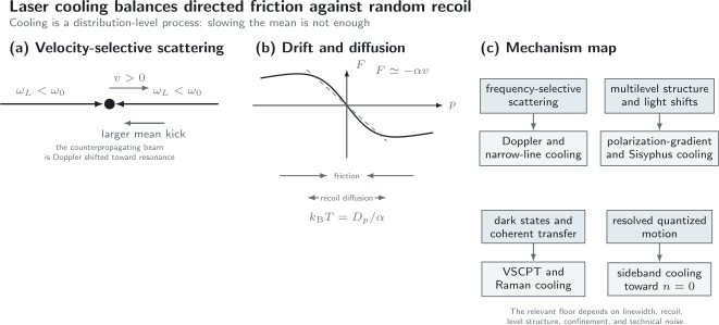
Cooling requires both a restoring drift in momentum space and an entropy sink. Red-detuned beams can generate $F\simeq-\alpha v$, while random photon recoil creates diffusion $D_p$. In the simplest one-dimensional Fokker–Planck limit, their balance gives $k_{\mathrm B}T=D_p/\alpha$. Multilevel structure, dark states, narrow transitions, and resolved quantized motion provide routes beyond the basic two-level Doppler regime.

Capture range

The linear force applies only near zero velocity. A rough spectral capture condition is

$$|kv| \lesssim \Gamma_{\mathrm{eff}},$$

where $\Gamma_{\mathrm{eff}}$ includes natural linewidth, power broadening, frequency modulation, field shifts, and the multilevel response. A force can have a steep damping slope but a narrow capture range.

Capture and final temperature are therefore different design objectives:

• broad transitions and high intensity improve force and capture;
• weak intensity and favorable detuning reduce the basic Doppler temperature;
• narrow transitions can reach lower temperatures but capture a smaller velocity class;
• staged cooling can combine a broad capture transition with a narrow final transition.

One beam is not optical molasses

A single beam generally produces a nonzero mean force even at $v=0$. It can slow atoms approaching from one direction, but it does not create symmetric damping around zero momentum. Counterpropagating beams create the local restoring drift in momentum space.

In three dimensions, six beams are a common idealization. Polarizations, magnetic fields, interference, beam imbalance, and multilevel optical pumping make the actual force more than three independent copies of the one-dimensional formula.

Friction–Diffusion Balance

Fokker–Planck model

Let $f(p,t)$ be a one-dimensional momentum distribution. Near the damping region, suppose

$$F = -\frac{\alpha}{m}p$$

and momentum kicks produce a constant diffusion coefficient $D_p$. The Fokker–Planck equation is

$$\frac{\partial f}{\partial t} = \frac{\alpha}{m} \frac{\partial}{\partial p} \left( pf \right) + D_p \frac{\partial^2f}{\partial p^2}.$$

The second moment obeys

$$\frac{d}{dt} \left\langle p^2\right\rangle = -\frac{2\alpha}{m} \left\langle p^2\right\rangle + 2D_p.$$

Hence the damping time for the momentum amplitude is

$$\tau_p = \frac{m}{\alpha},$$

while the kinetic-energy or variance relaxation has rate $2\alpha/m$ in this linear model.

At stationarity,

$$\left\langle p^2\right\rangle_{\mathrm{ss}} = \frac{mD_p}{\alpha}.$$

If the stationary distribution is thermal,

$$\left\langle p^2\right\rangle = mk_{\mathrm B}T,$$

so

$$k_{\mathrm B}T = \frac{D_p}{\alpha}.$$

What sets diffusion?

Momentum diffusion can include:

• random spontaneous-emission directions;
• fluctuations in absorption times;
• random choices among counterpropagating beams;
• state switching among different light shifts;
• dipole-force fluctuations;
• laser amplitude, phase, frequency, and pointing noise;
• collisions and reabsorption of scattered photons.

Computing only the damping coefficient cannot predict a temperature.

Tensor form

In several dimensions, friction and diffusion are tensors:

$$F_i \simeq -\sum_j\alpha_{ij}v_j,$$ $$\frac{d}{dt} \operatorname{Cov}(p_i,p_j) \bigg|_{\mathrm{diff}} = 2D_{ij}.$$

Anisotropic emission, polarization gradients, trap geometry, and magnetic fields can produce unequal temperatures and cross-correlations. Quoting one temperature is justified only after thermalization or an explicit averaging rule.

Benchmark Temperature and Energy Scales

Two-level Doppler scale

For weakly saturated, broad-line, two-level optical molasses, optimizing the standard friction–diffusion balance gives the benchmark

$$k_{\mathrm B}T_D = \frac{\hbar\Gamma}{2}.$$

Under the atom-minus-laser convention, the weak-saturation optimum occurs at

$$\Delta = \frac{\Gamma}{2}.$$

This Doppler limit is not a universal lower bound on laser cooling. It is the minimum of a specific semiclassical two-level model. Multilevel polarization-gradient cooling, dark-state methods, Raman cooling, resolved sideband cooling, and narrow transitions violate one or more assumptions of that model.

Recoil scale

The recoil temperature is

$$T_r = \frac{ \hbar^2k^2 }{ 2mk_{\mathrm B} }.$$

The ratio

$$\frac{T_D}{T_r} = \frac{\Gamma}{2\omega_r}$$

separates useful regimes.

• If $\Gamma\gg\omega_r$, many recoil steps fit within the optical linewidth, and a semiclassical momentum description is often effective.
• If $\Gamma$ is comparable to $\omega_r$, individual recoil and narrow-line effects become central.
• In a trap with resolved motional spacing, the relevant comparison includes $\omega_t/\Gamma_{\mathrm{eff}}$ and the Lamb–Dicke parameter.

The recoil temperature is also not an absolute lower bound. Dark states can protect particles near zero velocity from further scattering, and resolved sideband cooling can prepare a trapped oscillator near $n=0$. The correct floor is mechanism dependent.

Trap quantum

For a harmonic trap of angular frequency $\omega_t$,

$$E_n = \hbar\omega_t \left( n+\frac{1}{2} \right).$$

If the motional state is thermal,

$$\bar n = \frac{1}{ \exp( \hbar\omega_t/k_{\mathrm B}T )-1 }.$$

Near the ground state, $\bar n$ and the full $P_n$ distribution are more informative than a classical temperature.

Cooling Mechanism Map

Broad-line Doppler cooling

Two or more red-detuned beams create velocity damping. The method offers large force and capture range and often supplies the first cooling stage for neutral atoms, ions, and suitable molecules. Its ideal two-level temperature is set by $\hbar\Gamma$, while real outcomes depend on multilevel structure, beam geometry, intensity, magnetic fields, and diffusion.

Optical molasses is the near-zero-field, approximately force-balanced version. It cools velocity but is not a stable position trap.

Narrow-line cooling

An intercombination or other narrow transition reduces the Doppler scale because $\Gamma$ is smaller. The capture velocity and maximum force also shrink. Gravity, recoil, power broadening, frequency sweeps, and magnetic field gradients can become comparable to the optical scales.

Staged alkaline-earth cooling commonly uses a broad transition for capture and a narrow transition for the final temperature. This is an engineering response to the capture–temperature trade-off.

Polarization-gradient and Sisyphus cooling

Real atoms have Zeeman and hyperfine sublevels. Spatially varying polarization creates state-dependent light shifts and optical-pumping rates. Atoms can repeatedly climb light-shift hills and be pumped into a lower energy state near the top, transferring motional energy to scattered light.

This mechanism can cool below the two-level Doppler limit. Its scale depends on light shifts and recoil rather than only $\hbar\Gamma$. Magnetic fields, polarization errors, and level degeneracy are central rather than small corrections.

Dark-state and subrecoil cooling

Coherent superpositions can decouple from the light. If the dark condition is velocity selective, particles accumulate near a narrow momentum class and stop scattering there.

Velocity-selective coherent population trapping and Raman cooling can create subrecoil distributions. Such distributions may be non-Gaussian and nonergodic, so assigning one equilibrium temperature can conceal their structure.

Resolved sideband cooling

A trapped particle has quantized motional sidebands. In the resolved-sideband regime, a drive can preferentially remove one motional quantum on a red sideband, while optical pumping resets the internal state with a small probability of changing motion in the Lamb–Dicke regime.

The cycle is:

$$|g,n\rangle \longrightarrow |e,n-1\rangle \longrightarrow |g,n-1\rangle.$$

The state $|g,0\rangle$ is dark to the red sideband because no $n=-1$ state exists. Imperfect sideband resolution, recoil during reset, off-resonant carrier excitation, motional heating, and trap-frequency noise set the final $\bar n$.

Raman sideband and EIT-assisted cooling

Raman transitions can couple internal states while changing motion with controllable wavevector difference. Raman sideband cooling combines sideband-selective coherent transfer with dissipative optical pumping. Electromagnetically induced transparency can reshape the absorption spectrum to suppress carrier excitation while enhancing a cooling sideband.

These are not synonymous methods. Their level schemes, dark states, linewidths, and reset channels must be specified.

Cavity-assisted cooling

A cavity can make anti-Stokes scattering into a selected lossy mode more probable than Stokes scattering. The cavity output removes energy and carries information. This can cool particles without relying on a free-space closed cycling transition in the same way as ordinary Doppler cooling.

The relevant scales include cavity linewidth, recoil, coupling, detuning, mode profile, and measurement backaction. Cavity QED supplies the canonical emitter–mode coupling framework.

Molecular laser cooling

Molecules have rotational and vibrational branching. Direct cooling requires an approximately closed optical cycle plus repump lasers that return population from important leakage states. Angular-momentum dark states, Zeeman structure, parity, and hyperfine splittings shape both force and cooling.

If the probability to remain in the addressed manifold per scattered photon is $b$, survival after $N$ cycles is approximately

$$P_{\mathrm{surv}} = b^N.$$

For the tens of thousands of photons needed to slow a molecular beam, a seemingly small leakage probability can be fatal. Optical cycling quality is a quantitative requirement, not a binary label.

Capture, Cooling, and Final-State Design

A useful cooling sequence often has several stages.

Stage 1: increase accepted phase-space volume

Slowers, chirped light, broadened spectra, transverse cooling, and large capture beams bring particles into the region where later cooling works. Metrics include flux, capture velocity, loading rate, and loss.

Stage 2: dissipative capture

A magneto-optical trap or trapped-ion Doppler stage combines optical damping with confinement. Metrics include atom number, temperature, cloud size, density, loading time, lifetime, and magnetic-field sensitivity.

Stage 3: lower temperature or motional occupation

Polarization-gradient, narrow-line, Raman-sideband, EIT, or resolved-sideband methods reduce temperature or $\bar n$. Metrics include the full distribution, ground-state probability, anisotropy, and heating after the cooling light is removed.

Stage 4: transfer to a conservative science trap

Atoms may be transferred into optical dipole traps, tweezers, lattices, or magnetic traps. Transfer efficiency, differential light shifts, density, collisions, and adiabaticity can change the state. The temperature after transfer is not necessarily the temperature before transfer.

Stage 5: evaporative or sympathetic cooling

Laser cooling often supplies the phase-space density required for subsequent evaporative cooling or sympathetic cooling. These are not themselves laser-cooling mechanisms: evaporation removes energetic particles, while sympathetic cooling transfers energy to another species or component that acts as a refrigerant.

Worked Estimate: Slowing Rubidium

Consider $^{87}\mathrm{Rb}$ on a transition near $\lambda=780.24\ \mathrm{nm}$ with

$$\frac{\Gamma}{2\pi} \simeq 6.07\ \mathrm{MHz}, \qquad m \simeq 1.443\times10^{-25}\ \mathrm{kg}.$$

The wave number and recoil velocity are approximately

$$k = \frac{2\pi}{\lambda} \simeq 8.05\times10^6\ \mathrm{m^{-1}},$$ $$v_r = \frac{\hbar k}{m} \simeq 5.88\times10^{-3}\ \mathrm{m\,s^{-1}}.$$

Photon budget

Slowing from $300\ \mathrm{m\,s^{-1}}$ to rest requires the ideal directed absorption budget

$$N_\gamma \simeq \frac{300}{5.88\times10^{-3}} \simeq 5.1\times10^4.$$

That number immediately explains why a cooling transition must be extremely closed and why repumping matters.

Force and stopping length

The ideal saturated two-level acceleration ceiling is

$$a_{\max} = \frac{\hbar k\Gamma}{2m} \simeq 1.1\times10^5\ \mathrm{m\,s^{-2}}.$$

Constant maximum deceleration would stop the atoms over

$$\ell_{\min} = \frac{v_0^2}{2a_{\max}} \simeq 0.40\ \mathrm{m}.$$

The corresponding time is about $2.7\ \mathrm{ms}$. A real slower uses a smaller fraction of $a_{\max}$ to maintain stability and account for intensity, polarization, field, and multilevel imperfections.

Doppler tracking

The initial Doppler angular shift is

$$kv_0 \simeq 2.42\times10^9\ \mathrm{s^{-1}},$$

or about $385\ \mathrm{MHz}$ in ordinary frequency. This is far larger than the natural linewidth. The resonance must be followed, for example with a spatial Zeeman shift or a frequency chirp.

Recoil and Doppler scales

For these values,

$$T_r \simeq 0.181\ \mu\mathrm K, \qquad T_D \simeq 146\ \mu\mathrm K.$$

The broad transition has $T_D\gg T_r$, so the standard Doppler theory is semiclassical over much of its operating range. Sub-Doppler mechanisms are needed to approach the recoil scale.

This estimate is a scale audit, not a design for a complete rubidium slower. It omits branching, hyperfine repumping, transverse diffusion, laser linewidth, beam profile, magnetic geometry, and collisions.

How Cooling Is Measured

Time of flight

After release and ballistic expansion,

$$x(t) = x_0+v_0t.$$

The spatial variance is

$$\sigma_x^2(t) = \sigma_x^2(0) + 2t\,\operatorname{Cov}(x_0,v_0) + t^2\sigma_v^2.$$

The familiar fit

$$\sigma_x^2(t) = \sigma_x^2(0) + \frac{k_{\mathrm B}T}{m}t^2$$

assumes a thermal Gaussian velocity distribution, negligible position–velocity covariance, ballistic motion, known magnification, and an imaging point-spread function that has been accounted for.

Release and recapture

The trap is switched off for a variable time and restored. The recaptured fraction is compared with a model or simulation. The inference depends on trap geometry, depth, gravity, switching transients, collisions, and the initial spatial distribution. It is model-dependent thermometry.

Doppler-sensitive spectroscopy

A narrow probe maps velocity onto detuning through $\mathbf k\mathbin{\cdot}\mathbf v$. The measured line also contains natural, power, laser, transit, collision, and instrumental broadening. Line Shapes and Broadening owns the canonical convolution and linewidth framework.

Sideband thermometry

For a thermal harmonic mode in the Lamb–Dicke regime, the integrated red-to-blue sideband-strength ratio is

$$\frac{A_{\mathrm{red}}}{A_{\mathrm{blue}}} = \frac{\bar n}{\bar n+1}.$$

Thus

$$\bar n = \frac{ A_{\mathrm{red}}/A_{\mathrm{blue}} }{ 1-A_{\mathrm{red}}/A_{\mathrm{blue}} }.$$

The relation assumes a thermal distribution, comparable probe response, resolved sidebands, and a model for state preparation and detection.

Full distribution and cross-checks

For non-Gaussian states, report more than a fitted temperature:

• velocity or momentum histograms;
• central width and tail fraction;
• anisotropic temperatures;
• sideband populations;
• particle number and density;
• heating rate after cooling;
• dependence on detuning, intensity, magnetic field, and cooling duration.

Agreement among independent thermometers is a stronger result than a small number from one model fit.

Limitations and Noise Sources

Open transitions

Branching into dark states stops scattering. Repump lasers return selected states, but every additional level introduces detunings, polarization dependence, and possible dark superpositions.

Multilevel optical pumping

The two-level formula can fail even when one transition appears dominant. Zeeman and hyperfine populations evolve during cooling. Polarization gradients can provide beneficial sub-Doppler forces or unwanted dark states, depending on geometry and magnetic field.

Recoil diffusion

Spontaneous emission has zero mean momentum only under suitable symmetry. Its variance never vanishes. Directional reservoirs, cavities, dipole patterns, and multibeam absorption alter the diffusion tensor.

Magnetic fields

Stray fields shift Zeeman sublevels, destroy dark states, move resonance conditions, and set quantization axes. A magneto-optical trap intentionally uses a gradient; molasses stages often require that gradient to be switched off rapidly and residual fields compensated.

Laser noise

Frequency noise changes detuning and therefore force. Intensity noise changes scattering and light shifts. Polarization drift changes transition strengths. Pointing noise changes local intensity and wavevector. Relative phase noise is central for Raman and dark-state methods.

Density effects

Scattered photons can be reabsorbed, producing outward pressure and extra diffusion. Light-assisted collisions cause loss and heating. Collective emission, multiple scattering, and radiation trapping can invalidate an independent-particle force model.

Finite response and nonadiabatic motion

The steady scattering force assumes that the internal state follows the changing detuning. Very rapid motion, short pulses, frequency sweeps, or strongly modulated fields require time-dependent optical Bloch dynamics.

Trap and surface heating

After laser cooling, electric-field noise, technical trap noise, photon scattering, collisions, and fluctuating potentials can reheat motion. The final useful quantity may be the heating rate $d\bar n/dt$ or $dT/dt$, not the temperature at the end of the cooling pulse.

A Reliable Cooling Analysis

1. Define the cooled variable. State whether the target is free-particle velocity, one trap mode, all secular modes, rotation, or another degree of freedom.
2. Write the level scheme. Include branching states, repumps, dark states, polarizations, and magnetic fields.
3. Declare detuning conventions. Derive the Doppler sign rather than importing it.
4. Identify the entropy sink. Name spontaneous emission, cavity loss, optical pumping, or another reset.
5. Calculate drift and diffusion. A mean force alone does not give a temperature.
6. Estimate capture. Compare velocity, force, interaction time, beam size, and changing Doppler shift.
7. Compare scales. Record $\Gamma$, $\omega_r$, trap frequencies, Rabi frequencies, light shifts, recoil, and technical noise.
8. Model loss. Include branching, collisions, background gas, and finite trap depth.
9. Choose a thermometer. State its distribution and imaging assumptions.
10. Validate. Reverse detuning, vary cooling time and intensity, compare independent thermometers, and measure reheating.

Common Mistakes

Equating lower mean speed with lower temperature

A slowed beam may have the same or a larger velocity spread. Subtract the mean before computing random kinetic energy.

Treating spontaneous emission as harmless because its mean recoil is zero

Zero mean does not imply zero variance. Spontaneous recoil is a primary source of diffusion.

Calling the Doppler limit fundamental

$T_D=\hbar\Gamma/(2k_{\mathrm B})$ belongs to a weak-saturation, broad-line, two-level model. Many established methods cool below it.

Calling the recoil temperature an absolute floor

Dark-state and trapped-particle methods can produce subrecoil widths or ground-state occupation. Recoil remains part of the transition ledger, but the final-state mechanism can suppress further scattering.

Ignoring capture while optimizing the final temperature

A narrow, weak transition can have an excellent local damping temperature and capture almost none of the incoming distribution.

Treating optical molasses as a trap

Balanced molasses damps velocity near zero but does not provide stable position confinement by itself.

Adding saturated beam forces independently

Beams share the same populations and coherences. Independent rates are a controlled weak-saturation or incoherent approximation.

Reporting a temperature without a distribution model

Time-of-flight, Doppler spectroscopy, release–recapture, and sideband thermometry infer different aspects of motion and rely on different assumptions.

Assuming every scattered photon remains in the cycle

For large $N_\gamma$, tiny branching probabilities accumulate. Repump completeness must be computed.

Connections

• AMO Platforms and Quantum Control places cooling inside the full preparation–control–measurement cycle.
• Alkali Atoms explains the level structures behind many common cooling transitions.
• Atomic Selection Rules gives the angular-momentum and polarization logic behind cycling and leakage.
• Cold Molecules applies photon-budget closure, repumping, and dark-state control to molecular cooling and compares it with assembly from ultracold atoms.
• Cavity QED supplies the coherent and dissipative scales for cavity-assisted cooling.
• Laser Cooling Simulation Notebook makes the simple Doppler force, friction–diffusion balance, convergence tests, and rubidium scale conversion executable.
• AMO Experiment Index distinguishes proposal, thermometry record, cooling mechanism, and historical milestone.
• Quantum Noise supplies the correlation and spectral language for force fluctuations.

References

1. T. W. Hänsch and A. L. Schawlow, “Cooling of gases by laser radiation,” Optics Communications 13, 68–69 (1975), doi:10.1016/0030-4018(75)90159-5.
2. D. J. Wineland and W. M. Itano, “Laser cooling of atoms,” Physical Review A 20, 1521–1540 (1979), doi:10.1103/PhysRevA.20.1521.
3. J. P. Gordon and A. Ashkin, “Motion of atoms in a radiation trap,” Physical Review A 21, 1606–1617 (1980), doi:10.1103/PhysRevA.21.1606.
4. S. Chu, “Nobel Lecture: The manipulation of neutral particles,” Reviews of Modern Physics 70, 685–706 (1998), doi:10.1103/RevModPhys.70.685.
5. C. N. Cohen-Tannoudji, “Nobel Lecture: Manipulating atoms with photons,” Reviews of Modern Physics 70, 707–719 (1998), doi:10.1103/RevModPhys.70.707.
6. W. D. Phillips, “Nobel Lecture: Laser cooling and trapping of neutral atoms,” Reviews of Modern Physics 70, 721–741 (1998), doi:10.1103/RevModPhys.70.721.
7. H. J. Metcalf and P. van der Straten, Laser Cooling and Trapping (Springer, 1999).
8. P. D. Lett, R. N. Watts, C. I. Westbrook, W. D. Phillips, P. L. Gould, and H. J. Metcalf, “Observation of atoms laser cooled below the Doppler limit,” Physical Review Letters 61, 169–172 (1988), doi:10.1103/PhysRevLett.61.169.
9. J. Dalibard and C. Cohen-Tannoudji, “Laser cooling below the Doppler limit by polarization gradients: simple theoretical models,” Journal of the Optical Society of America B 6, 2023–2045 (1989), doi:10.1364/JOSAB.6.002023.
10. Y. Castin, H. Wallis, and J. Dalibard, “Limit of Doppler cooling,” Journal of the Optical Society of America B 6, 2046–2057 (1989), doi:10.1364/JOSAB.6.002046.
11. A. Aspect, E. Arimondo, R. Kaiser, N. Vansteenkiste, and C. Cohen-Tannoudji, “Laser cooling below the one-photon recoil energy by velocity-selective coherent population trapping,” Physical Review Letters 61, 826–829 (1988), doi:10.1103/PhysRevLett.61.826.
12. M. Kasevich and S. Chu, “Laser cooling below a photon recoil with three-level atoms,” Physical Review Letters 69, 1741–1744 (1992), doi:10.1103/PhysRevLett.69.1741.
13. F. Diedrich, J. C. Bergquist, W. M. Itano, and D. J. Wineland, “Laser cooling to the zero-point energy of motion,” Physical Review Letters 62, 403–406 (1989), doi:10.1103/PhysRevLett.62.403.
14. D. Leibfried, R. Blatt, C. Monroe, and D. Wineland, “Quantum dynamics of single trapped ions,” Reviews of Modern Physics 75, 281–324 (2003), doi:10.1103/RevModPhys.75.281.
15. H. Katori, T. Ido, Y. Isoya, and M. Kuwata-Gonokami, “Magneto-optical trapping and cooling of strontium atoms down to the photon recoil temperature,” Physical Review Letters 82, 1116–1119 (1999), doi:10.1103/PhysRevLett.82.1116.
16. E. S. Shuman, J. F. Barry, and D. DeMille, “Laser cooling of a diatomic molecule,” Nature 467, 820–823 (2010), doi:10.1038/nature09443.
17. C. Cohen-Tannoudji and D. Guéry-Odelin, Advances in Atomic Physics: An Overview (World Scientific, 2011).

Exercises

1. Slowing is not cooling

Two one-dimensional atomic beams have velocity distributions:

$$v_A = (300\pm20)\ \mathrm{m\,s^{-1}},$$ $$v_B = (30\pm25)\ \mathrm{m\,s^{-1}},$$

where the numbers after $\pm$ are one-standard-deviation widths. The atomic mass is the same.

1. Which beam is slower?
2. Which beam has the lower variance temperature?
3. By what factor do their one-dimensional variance temperatures differ?

Solution

Beam B has the lower mean speed, so it is slower in the laboratory.

The variance temperature is

$$k_{\mathrm B}T^{(\mathrm{var})} = m\sigma_v^2.$$

Beam A has $\sigma_A=20\ \mathrm{m\,s^{-1}}$ and beam B has $\sigma_B=25\ \mathrm{m\,s^{-1}}$. Therefore A is colder by this measure, despite moving faster on average.

The ratio is

$$\frac{T_B}{T_A} = \frac{\sigma_B^2}{\sigma_A^2} = \left(\frac{25}{20}\right)^2 = 1.5625.$$

Beam B is slower but has a $56\%$ larger variance temperature.

2. Photon momentum budget

For $^{87}\mathrm{Rb}$ at $780.24\ \mathrm{nm}$, use $v_r=5.88\ \mathrm{mm\,s^{-1}}$.

1. How many directed absorption events are required to change the atomic speed by $50\ \mathrm{m\,s^{-1}}$?
2. If spontaneous emission is isotropic and independent, estimate the rms velocity diffusion in one transverse direction after this many events.

Solution

The ideal number is

$$N = \frac{50}{5.88\times10^{-3}} \simeq 8.50\times10^3.$$

For isotropic emission, one Cartesian component has mean-square recoil $v_r^2/3$ per event. Independent events add variances:

$$\sigma_{v_\perp} \simeq v_r\sqrt{\frac{N}{3}}.$$

Thus

$$\sigma_{v_\perp} \simeq (5.88\times10^{-3}) \sqrt{\frac{8.50\times10^3}{3}} \simeq 0.313\ \mathrm{m\,s^{-1}}.$$

Directed slowing therefore coexists with transverse recoil diffusion. Dipole emission patterns and absorption from multiple beams modify the numerical factor.

3. Friction sign

In the weak-saturation model,

$$F(v) = \hbar k \left[ R(\Delta+kv)-R(\Delta-kv) \right],$$

where

$$R(\delta) = \frac{\Gamma s_0/2}{ 1+(2\delta/\Gamma)^2 }.$$

Show that red detuning under the convention $\Delta=\omega_0-\omega_L>0$ produces $F\simeq-\alpha v$ with $\alpha>0$.

Solution

Expand about $v=0$:

$$R(\Delta\pm kv) \simeq R(\Delta) \pm kvR'(\Delta).$$

Therefore

$$F(v) \simeq 2\hbar k^2vR'(\Delta).$$

Differentiating,

$$R'(\Delta) = -\frac{ 4s_0(\Delta/\Gamma) }{ \left[ 1+(2\Delta/\Gamma)^2 \right]^2 }.$$

Hence

$$F(v) \simeq -\alpha v,$$

with

$$\alpha = 8\hbar k^2s_0 \frac{ \Delta/\Gamma }{ \left[ 1+(2\Delta/\Gamma)^2 \right]^2 }.$$

For $\Delta>0$, $\alpha>0$. The force opposes small velocity. A source using laser-minus-atom detuning assigns the opposite sign to red detuning.

4. Cooling time and steady variance

The one-dimensional momentum distribution obeys

$$\frac{\partial f}{\partial t} = \frac{\alpha}{m} \frac{\partial}{\partial p}(pf) + D_p\frac{\partial^2f}{\partial p^2}.$$

Given initial variance $V_0=\langle p^2\rangle_0$, solve for $V(t)=\langle p^2\rangle_t$ and identify the stationary temperature.

Solution

The second moment obeys

$$\dot V = -\frac{2\alpha}{m}V+2D_p.$$

The solution is

$$V(t) = \frac{mD_p}{\alpha} + \left( V_0-\frac{mD_p}{\alpha} \right) \exp\left( -\frac{2\alpha t}{m} \right).$$

The stationary variance is

$$V_{\mathrm{ss}} = \frac{mD_p}{\alpha}.$$

For a thermal one-dimensional distribution, $V_{\mathrm{ss}}=mk_{\mathrm B}T$, so

$$k_{\mathrm B}T = \frac{D_p}{\alpha}.$$

The variance relaxes with time constant $m/(2\alpha)$, while the mean momentum relaxes with time constant $m/\alpha$.

5. Doppler versus recoil scales

For the rubidium-like values

$$\frac{\Gamma}{2\pi} = 6.07\ \mathrm{MHz}, \qquad \frac{\omega_r}{2\pi} = 3.77\ \mathrm{kHz},$$

compute $T_D/T_r$. What does the result imply?

Solution

Using

$$\frac{T_D}{T_r} = \frac{\Gamma}{2\omega_r},$$

ordinary-frequency factors of $2\pi$ cancel:

$$\frac{T_D}{T_r} = \frac{6.07\times10^6}{ 2(3.77\times10^3) } \simeq 805.$$

The natural linewidth is much larger than the recoil frequency. The two-level Doppler scale lies hundreds of recoil temperatures above $T_r$. This supports a semiclassical broad-line description over the Doppler stage and leaves substantial room for sub-Doppler cooling.

6. Time-of-flight covariance

A released cloud has

$$\sigma_x(0)=0.20\ \mathrm{mm}, \qquad \sigma_v=0.030\ \mathrm{m\,s^{-1}},$$

and

$$\operatorname{Cov}(x_0,v_0) = -3.0\times10^{-6}\ \mathrm{m^2\,s^{-1}}.$$

Find $\sigma_x$ after $t=10\ \mathrm{ms}$. Compare with a fit that neglects the covariance.

Solution

The full variance is

$$\sigma_x^2(t) = \sigma_x^2(0) + 2t\,\operatorname{Cov}(x_0,v_0) + t^2\sigma_v^2.$$

The three terms are

$$\sigma_x^2(0) = 4.0\times10^{-8}\ \mathrm{m^2},$$ $$2t\,\operatorname{Cov} = -6.0\times10^{-8}\ \mathrm{m^2},$$ $$t^2\sigma_v^2 = 9.0\times10^{-8}\ \mathrm{m^2}.$$

Thus

$$\sigma_x^2(t) = 7.0\times10^{-8}\ \mathrm{m^2},$$

and

$$\sigma_x(t) \simeq 0.265\ \mathrm{mm}.$$

Neglecting covariance would give

$$\sigma_x^2 = 1.30\times10^{-7}\ \mathrm{m^2}, \qquad \sigma_x \simeq 0.361\ \mathrm{mm}.$$

The inferred velocity width and temperature would be biased upward. A position–velocity correlation can arise from focusing, trap switching, or nonequilibrium dynamics.

7. How closed must a transition be?

A slowing stage requires $N=5.0\times10^4$ scattered photons. Let $b$ be the probability per photon that the particle remains in the addressed cycling manifold.

1. If $b=0.9999$, what fraction survives?
2. What minimum $b$ is required for $90\%$ survival?

Solution

The survival probability is

$$P=b^N.$$

For $b=0.9999$,

$$P = (0.9999)^{50000} \simeq \exp(-5.000) \simeq 6.7\times10^{-3}.$$

Only about $0.67\%$ survive.

For $P=0.90$,

$$b = P^{1/N} = \exp\left( \frac{\ln0.90}{50000} \right) \simeq 0.99999789.$$

The allowed leakage probability per photon is only about $2.1\times10^{-6}$. This is why apparently weak vibrational or hyperfine branching requires repumping.

8. Sideband thermometry

A trapped particle has an integrated red-to-blue sideband ratio

$$r = \frac{A_{\mathrm{red}}}{A_{\mathrm{blue}}} = 0.12.$$

Assuming a thermal motional state in the Lamb–Dicke regime, find $\bar n$ and the ground-state probability $P_0$.

Solution

The sideband ratio gives

$$r = \frac{\bar n}{\bar n+1}.$$

Therefore

$$\bar n = \frac{r}{1-r} = \frac{0.12}{0.88} \simeq 0.136.$$

For a thermal harmonic oscillator,

$$P_n = \frac{1}{\bar n+1} \left( \frac{\bar n}{\bar n+1} \right)^n.$$

Thus

$$P_0 = \frac{1}{\bar n+1} \simeq 0.880.$$

The inference should be qualified if the motional distribution is nonthermal, the sidebands overlap, or probe saturation differs between red and blue scans.