Radiation Pressure

Radiation pressure is mechanical momentum transfer from an electromagnetic field to matter. For a freely moving atom, a photon absorbed from a traveling wave changes the atomic momentum by $+\hbar\mathbf k$. Subsequent spontaneous emission gives a recoil $-\hbar\mathbf k_s$, so one complete scattering cycle changes the atomic momentum by

$$\Delta\mathbf p = \hbar \left( \mathbf k-\mathbf k_s \right).$$

In free space, the mean spontaneous-emission direction often vanishes. The mean cycle impulse is then $\hbar\mathbf k$, directed along the incident beam. The emitted direction still fluctuates, so the same cycles that produce a mean force also produce momentum diffusion and recoil heating.

For a closed two-level atom driven by one traveling wave, the steady scattering force is

$$\mathbf F_{\mathrm{sc}} = \hbar\mathbf k \frac{\Gamma}{2} \frac{ s_0 }{ 1+s_0+ \left( 2\Delta_v/\Gamma \right)^2 }.$$

Here $\Gamma$ is the excited-state population decay rate, $s_0=2|\Omega|^2/\Gamma^2$ is the on-resonance saturation parameter, and $\Delta_v$ is the Doppler-shifted detuning. This compact expression is powerful, but its assumptions matter: a closed transition, a stationary internal state, one traveling mode, controlled recoil averaging, and center-of-mass motion slow enough that the internal steady state can follow.

Radiation pressure is not synonymous with every optical force. The dissipative scattering force follows the beam’s phase gradient and requires irreversible emission. The conservative dipole force follows an intensity gradient and is generated by a position-dependent light shift. Real laser fields can exert both.

Canonical Scope

This page owns:

1. the momentum ledger for absorption, stimulated emission, and spontaneous emission;
2. the mean scattering force of a driven two-level atom;
3. saturation, resonant cross section, and the maximum force;
4. Doppler-shifted force and the low-velocity damping slope;
5. recoil, momentum diffusion, and mechanical heating;
6. the distinction between scattering and dipole forces;
7. multibeam, multilevel, cavity, and experimental limitations;
8. the mechanical bridge to laser cooling without re-deriving cooling temperatures or trap architectures.

Nearby canonical homes remain distinct:

• Photon Momentum owns the historical evidence, the classical field-momentum connection, and the relation $p_\gamma=h/\lambda$.
• Optical Bloch Equations owns the driven density-matrix dynamics, steady-state population, and saturation derivation used here.
• Spontaneous Emission owns the radiative decay rate, angular pattern, branching, and environment dependence.
• AC Stark Shift and Dynamic Polarizability own conservative light shifts, dipole potentials, and multilevel polarizabilities.
• Quantum-Jump Trajectories owns state evolution conditioned on individual emission records.
• Optomechanics owns radiation-pressure coupling to a retained cavity mode, dynamical backaction, and measurement noise.

This page treats the center-of-mass mechanics of a laser-driven atom and cross-links rather than duplicating those subjects.

From Energy Flux to Pressure

Classical benchmark

A plane wave of intensity $I$ carries energy flux $I$ and momentum flux $I/c$ in vacuum. At normal incidence, an ideal absorbing surface therefore feels pressure

$$P_{\mathrm{abs}} = \frac{I}{c}.$$

A perfectly reflecting surface reverses the normal momentum and feels

$$P_{\mathrm{refl}} = \frac{2I}{c}.$$

Radiation pressure therefore does not by itself prove that the field is in a photon-number state. Classical Maxwell fields carry momentum. The photon description becomes especially useful when individual absorption and emission recoils, counting fluctuations, and internal transitions must be tracked.

Atomic effective area

An atom does not present a hard geometric disk. Near an allowed resonance, its optical response defines a frequency-, polarization-, state-, and intensity-dependent effective cross section. In the weak-field limit, the force can be written

$$F_{\mathrm{sc}} = \frac{I}{c} \sigma(\Delta_v).$$

This has the same momentum-flux structure as macroscopic pressure, but the atomic cross section can be much larger than the atom’s geometric area. Saturation eventually makes the response nonlinear in $I$.

Photon Momentum Ledger

Absorption

For a traveling mode with wave vector $\mathbf k$, absorption removes one field quantum of momentum $\hbar\mathbf k$. Momentum conservation gives

$$\Delta\mathbf p_{\mathrm{atom}}^{\mathrm{abs}} = +\hbar\mathbf k.$$

The statement assumes that any momentum supplied to an optical element, substrate, or second field has already been included in the chosen system boundary.

Stimulated emission

Stimulated emission into the same traveling mode adds a photon with momentum $\hbar\mathbf k$ to that mode. The atom receives

$$\Delta\mathbf p_{\mathrm{atom}}^{\mathrm{stim}} = -\hbar\mathbf k.$$

Absorption and stimulated emission therefore push in opposite directions. It is incorrect to count every coherent excitation as a permanent $+\hbar\mathbf k$ impulse while ignoring stimulated return.

Spontaneous emission

If the emitted photon has wave vector $\mathbf k_s$, the atomic recoil is

$$\Delta\mathbf p_{\mathrm{atom}}^{\mathrm{sp}} = -\hbar\mathbf k_s.$$

For one absorption–spontaneous-emission cycle,

$$\Delta\mathbf p_{\mathrm{cycle}} = \hbar\mathbf k - \hbar\mathbf k_s.$$

The emitted photon is not generally isotropic. Electric-dipole radiation has an angular pattern fixed by the transition and polarization. In inversion-symmetric free space one often has

$$\left\langle \mathbf k_s \right\rangle = 0,$$

even though the second moment is nonzero. Cavities, waveguides, nearby surfaces, collective emission, or chiral coupling can make the mean emission recoil directional.

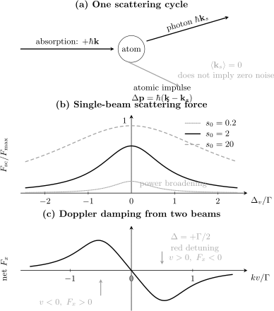
Top: absorption supplies $+\hbar\mathbf k$ and spontaneous emission supplies $-\hbar\mathbf k_s$. Middle: the single-beam force is a power-broadened, saturating resonance. Bottom: two weak counterpropagating red-detuned beams produce a net force opposing small velocities, while recoil fluctuations remain.

Force as Momentum Transfer Rate

Ehrenfest form

Let $\mathbf R$ and $\mathbf P$ be the center-of-mass position and canonical momentum. For an interaction Hamiltonian $H_{\mathrm{int}}(\mathbf R)$, the optical force operator is

$$\widehat{\mathbf F} = - \boldsymbol\nabla_{\mathbf R} H_{\mathrm{int}}.$$

Ehrenfest’s theorem gives

$$\frac{d}{dt} \left\langle \mathbf P \right\rangle = \left\langle \widehat{\mathbf F} \right\rangle$$

when no other external force is present. A traveling wave contains both an amplitude gradient and a phase gradient. Differentiating the light–matter Hamiltonian separates:

• an amplitude-gradient contribution associated with the reactive dipole force;
• a phase-gradient contribution associated with directed momentum transfer.

The cycle picture and the force-operator picture are two descriptions of the same momentum conservation. The cycle picture is particularly transparent after spontaneous events can be treated as resolved or coarse-grained jumps.

Steady-state balance

Let $R_{\mathrm{abs}}$ and $R_{\mathrm{stim}}$ denote the net upward and stimulated downward rates in a rate description. For a closed two-level transition,

$$\dot\rho_{ee} = R_{\mathrm{abs}} - R_{\mathrm{stim}} - \Gamma\rho_{ee}.$$

At steady state,

$$R_{\mathrm{abs}} - R_{\mathrm{stim}} = \Gamma\rho_{ee}^{\mathrm{ss}}.$$

The net rate at which directed photons are removed from the traveling beam equals the spontaneous-emission rate. If the mean spontaneous recoil is zero,

$$\mathbf F_{\mathrm{sc}} = \hbar\mathbf k \Gamma\rho_{ee}^{\mathrm{ss}}.$$

In a coherently driven atom, absorption and stimulated emission need not admit a unique trajectory decomposition at every instant. The steady-state balance above is the operational statement needed for the mean force.

Closed Two-Level Scattering Force

Conventions

Use a closed transition $|g\rangle\leftrightarrow|e\rangle$ with angular frequency $\omega_0$, population decay rate $\Gamma$, and a plane-wave laser with angular frequency $\omega_L$ and wave vector $\mathbf k$. This chapter uses atom-minus-laser detuning:

$$\Delta = \omega_0-\omega_L.$$

Red detuning has $\Delta>0$. All frequencies and decay rates are angular quantities unless divided by $2\pi$.

The Rabi Hamiltonian contains the off-diagonal coefficient $\hbar\Omega/2$. Define the on-resonance saturation parameter

$$s_0 = \frac{ 2|\Omega|^2 }{ \Gamma^2 }.$$

Doppler detuning

For a nonrelativistic atom with velocity $\mathbf v$, the laser frequency in the atomic rest frame is

$$\omega_L' \simeq \omega_L - \mathbf k\mathbin{\cdot}\mathbf v.$$

The effective detuning is therefore

$$\Delta_v = \Delta + \mathbf k\mathbin{\cdot}\mathbf v.$$

Writing the optical phase and transforming it is safer than memorizing a Doppler sign. A reference using laser-minus-atom detuning displays the opposite sign.

Steady excited-state population

The optical Bloch steady state gives

$$\rho_{ee}^{\mathrm{ss}} = \frac12 \frac{ s_0 }{ 1+s_0+ \left( 2\Delta_v/\Gamma \right)^2 }.$$

It is also useful to define the detuning-dependent saturation parameter

$$s(\Delta_v) = \frac{ s_0 }{ 1+ \left( 2\Delta_v/\Gamma \right)^2 }.$$

Then

$$\rho_{ee}^{\mathrm{ss}} = \frac{ s }{ 2(1+s) }.$$

Scattering rate

The spontaneous scattering rate is

$$R_{\mathrm{sc}} = \Gamma\rho_{ee}^{\mathrm{ss}},$$

or

$$R_{\mathrm{sc}} = \frac{\Gamma}{2} \frac{ s_0 }{ 1+s_0+ \left( 2\Delta_v/\Gamma \right)^2 }.$$

The corresponding mean force is

$$\mathbf F_{\mathrm{sc}} = \hbar\mathbf k R_{\mathrm{sc}}.$$

This result assumes the mean emitted momentum vanishes. If it does not, replace the impulse per cycle:

$$\mathbf F = \hbar \left( \mathbf k - \left\langle \mathbf k_s \right\rangle \right) R_{\mathrm{sc}}.$$

Saturation and Force Limits

Maximum rate and force

On resonance,

$$R_{\mathrm{sc}}(0) = \frac{\Gamma}{2} \frac{ s_0 }{ 1+s_0 }.$$

As $s_0\to\infty$,

$$\rho_{ee}^{\mathrm{ss}} \longrightarrow \frac12,$$

and

$$R_{\mathrm{sc}} \longrightarrow \frac{\Gamma}{2}.$$

The ideal two-level force is bounded by

$$F_{\max} = \frac{ \hbar k\Gamma }{ 2 }.$$

The associated maximum acceleration is

$$a_{\max} = \frac{ \hbar k\Gamma }{ 2m }.$$

Increasing intensity far beyond saturation does not make a closed two-level atom scatter arbitrarily fast. The atom spends approximately half its time excited, and stimulated emission competes with absorption.

Power broadening

The force profile is Lorentzian in $\Delta_v$ with a saturated half-width

$$\Delta_{\mathrm{HWHM}} = \frac{\Gamma}{2} \sqrt{ 1+s_0 }.$$

Intensity therefore changes both the peak and the velocity or frequency range over which the force is substantial. A broadened force profile is not evidence that $\Gamma$ itself increased.

Response-time condition

The steady formula assumes that position, velocity, intensity, detuning, and polarization vary slowly enough for the internal state to relax toward the local steady state. A short pulse or rapid transit requires time-dependent optical Bloch evolution and the impulse

$$\Delta\mathbf p = \int_{t_i}^{t_f} \mathbf F(t)\,dt.$$

A coherent $\pi$ pulse can transfer approximately one photon recoil, but repeated dissipative force requires a mechanism that resets the internal state.

Resonant Cross Section

Weak-field form

The photon flux in a plane wave is

$$\Phi_\gamma = \frac{ I }{ \hbar\omega_L }.$$

In the weak-field limit,

$$R_{\mathrm{sc}} = \Phi_\gamma \sigma(\Delta_v).$$

For an ideal closed electric-dipole transition with the appropriate polarization and degeneracy assumptions,

$$\sigma_0 = \frac{ 3\lambda^2 }{ 2\pi },$$

and

$$\sigma(\Delta_v) = \frac{ \sigma_0 }{ 1+ \left( 2\Delta_v/\Gamma \right)^2 }.$$

Then

$$F_{\mathrm{sc}} = \frac{I}{c} \sigma(\Delta_v).$$

This directly connects the photon-cycle result to incident momentum flux.

Saturation intensity

Define $I_{\mathrm{sat}}$ by

$$s_0 = \frac{I}{I_{\mathrm{sat}}}.$$

For the same ideal cycling transition and conventions,

$$I_{\mathrm{sat}} = \frac{ \pi h c\Gamma }{ 3\lambda^3 }.$$

At finite intensity one may write an effective nonlinear cross section

$$\sigma_{\mathrm{eff}} = \frac{ \sigma_0 }{ 1+s_0+ \left( 2\Delta_v/\Gamma \right)^2 },$$

so that $F=I\sigma_{\mathrm{eff}}/c$. This is bookkeeping for saturation, not a linear material cross section independent of the incident field.

Real-atom corrections

The familiar $\sigma_0$ and $I_{\mathrm{sat}}$ require a declared transition. Real corrections include:

• Clebsch–Gordan coefficients and laser polarization;
• ground- and excited-state degeneracy;
• branching into states outside the driven cycle;
• optical pumping among Zeeman or hyperfine levels;
• imperfect spatial mode and intensity calibration;
• laser linewidth and frequency noise;
• nearby transitions and interference;
• collective and propagation effects.

Quoting a universal saturation intensity without the transition, polarization, and state preparation is incomplete.

A Rubidium-Like Estimate

Consider a cycling transition with rounded parameters

$$\begin{aligned} \lambda &= 780\ \mathrm{nm}, \\ \frac{\Gamma}{2\pi} &= 6.0\ \mathrm{MHz}, \\ m &= 1.44\times10^{-25}\ \mathrm{kg}. \end{aligned}$$

Take

$$s_0=2, \qquad \Delta=\frac{\Gamma}{2}, \qquad v=0.$$

The force denominator is

$$1+s_0+ \left( 2\Delta/\Gamma \right)^2 = 4,$$

so

$$R_{\mathrm{sc}} = \frac{\Gamma}{4} \simeq 9.4\times10^6\ \mathrm{s^{-1}}.$$

The photon recoil momentum is

$$\hbar k = \frac{h}{\lambda} \simeq 8.5\times10^{-28}\ \mathrm{kg\,m\,s^{-1}}.$$

Hence

$$\begin{aligned} F_{\mathrm{sc}} &\simeq 8.0\times10^{-21}\ \mathrm N, \\ a &\simeq 5.6\times10^4\ \mathrm{m\,s^{-2}}. \end{aligned}$$

The force is microscopic, but the mass is smaller still. During $10\ \mathrm{\mu s}$, a constant-force estimate gives approximately

$$N_{\mathrm{sc}} = R_{\mathrm{sc}}t \simeq 94$$

cycles and a speed change

$$\Delta v \simeq N_{\mathrm{sc}} \frac{\hbar k}{m} \simeq 0.56\ \mathrm{m\,s^{-1}}.$$

This estimate must be audited for Doppler feedback. At the predicted final speed,

$$\frac{k\Delta v}{\Gamma} \simeq 0.12.$$

The atom has moved measurably across the force profile, so even this short constant-force estimate is only approximate. Over longer slowing times, laser chirping or a position-dependent Zeeman shift is needed to maintain resonance.

Recoil Scales

Single-photon recoil

Define

$$p_r = \hbar k,$$

the recoil velocity

$$v_r = \frac{ \hbar k }{ m },$$

and the recoil energy

$$E_r = \frac{ \hbar^2k^2 }{ 2m }.$$

The recoil angular frequency is

$$\omega_r = \frac{E_r}{\hbar}.$$

These scales determine when center-of-mass motion must be quantized rather than treated as a continuous classical trajectory.

Energy per scattering cycle

For absorption from fixed $\mathbf k$ followed by free-space emission with $|\mathbf k_s|\simeq k$ and $\langle\mathbf k_s\rangle=0$,

$$\left\langle |\Delta\mathbf p|^2 \right\rangle = 2\hbar^2k^2.$$

The corresponding recoil contribution to kinetic energy is

$$\frac{ \left\langle |\Delta\mathbf p|^2 \right\rangle }{ 2m } = 2E_r$$

per independent cycle. The total energy change also contains mechanical work from the mean force:

$$\dot E_{\mathrm{kin}} = \mathbf F\mathbin{\cdot}\mathbf v + \text{diffusive heating}.$$

Directed acceleration and random heating are different moments of the same recoil process.

Momentum Diffusion

Covariance growth

Let $\mathbf u$ be a unit vector along a measured axis. In an independent-cycle model,

$$\begin{aligned} \frac{d}{dt} \operatorname{Var}(p_u) = \hbar^2R_{\mathrm{sc}} \Big[ & \left( \mathbf u\mathbin{\cdot}\mathbf k \right)^2 \\ &+ \left\langle \left( \mathbf u\mathbin{\cdot}\mathbf k_s \right)^2 \right\rangle \Big]. \end{aligned}$$

The first term is absorption-number noise along the incident beam. The second is random spontaneous-emission recoil. If a Fokker–Planck equation uses

$$\frac{d}{dt} \operatorname{Var}(p_u) = 2D_{p,u},$$

then

$$\begin{aligned} D_{p,u} = \frac{\hbar^2R_{\mathrm{sc}}}{2} \Big[ & \left( \mathbf u\mathbin{\cdot}\mathbf k \right)^2 \\ &+ \left\langle \left( \mathbf u\mathbin{\cdot}\mathbf k_s \right)^2 \right\rangle \Big]. \end{aligned}$$

Authors also use a convention without the factor of two. A quoted momentum diffusion coefficient is ambiguous until its defining equation is stated.

Isotropic-emission example

For isotropic emission,

$$\left\langle \left( \mathbf u\mathbin{\cdot}\mathbf k_s \right)^2 \right\rangle = \frac{k^2}{3}.$$

Along the incident beam,

$$\frac{d}{dt} \operatorname{Var}(p_\parallel) = \frac43 \hbar^2k^2 R_{\mathrm{sc}}.$$

Electric-dipole emission is not generally isotropic, so the factor $1/3$ must be replaced by the angular moment of the actual radiation pattern.

Beyond independent cycles

At high saturation or in structured fields, the simple Poisson-cycle model can miss:

• antibunching and temporal correlations in resonance fluorescence;
• fluctuations of the coherent dipole force;
• standing-wave position dependence;
• internal-state switching;
• cavity-modified emission;
• collective scattering and reabsorption.

The mean force can remain accurate while its noise model fails. Mechanical heating, linewidths, and trap loss depend on the second moments.

Scattering Force and Dipole Force

Reactive optical potential

For a far-detuned, slowly varying two-level field, the ground-state light shift in this chapter’s detuning convention is

$$U_g(\mathbf r) \simeq - \frac{ \hbar|\Omega(\mathbf r)|^2 }{ 4\Delta }.$$

The conservative dipole force is

$$\mathbf F_{\mathrm{dip}} = - \boldsymbol\nabla U_g.$$

For red detuning, $\Delta>0$, this ideal ground state is attracted toward larger intensity.

Dissipative rate

In the same weak, far-detuned limit,

$$R_{\mathrm{sc}} \simeq \frac{ \Gamma|\Omega|^2 }{ 4\Delta^2 }.$$

The light shift scales as $I/\Delta$, while scattering scales as $I/\Delta^2$. Increasing detuning at fixed trap depth reduces the scattering cost in the ideal one-line model, but finite power and multilevel structure limit that strategy.

Operational distinction

Property	Scattering force	Dipole force
response	absorptive or dissipative	dispersive or reactive
direction	optical phase gradient, often $\mathbf k$	intensity or dressed-energy gradient
steady origin	irreversible photon redistribution	position-dependent light shift
saturation	bounded by the internal cycling rate	depends on dressed potential and adiabaticity
fluctuations	photon recoil and force noise are intrinsic	technical and quantum fluctuations can remain
uniform plane wave	generally nonzero near resonance	zero if amplitude is uniform

A focused beam can exert both forces simultaneously. Calling the total force “radiation pressure” without specifying its dissipative and conservative parts can hide the relevant physics.

Counterpropagating Beams

Weak-saturation model

Consider two equal, incoherently added traveling waves along $\pm x$, each with on-resonance saturation parameter $s_0\ll1$. For velocity $v$ along $+x$, their detunings are

$$\Delta_+ = \Delta+kv,$$

and

$$\Delta_- = \Delta-kv.$$

The low-saturation net force is

$$\begin{aligned} F(v) = \frac{\hbar k\Gamma s_0}{2} \Bigg[ & \frac{ 1 }{ 1+ \left( 2\Delta_+/\Gamma \right)^2 } \\ &- \frac{ 1 }{ 1+ \left( 2\Delta_-/\Gamma \right)^2 } \Bigg]. \end{aligned}$$

At $v=0$, the two forces cancel.

Low-velocity damping

For $|kv|\ll\Gamma$, expand:

$$F(v) \simeq -\alpha v.$$

The friction coefficient is

$$\alpha = \frac{ 8\hbar k^2s_0 \left( \Delta/\Gamma \right) }{ \left[ 1+ \left( 2\Delta/\Gamma \right)^2 \right]^2 }.$$

With this page’s convention, red detuning has $\Delta>0$, so $\alpha>0$ and the force opposes small velocities. Blue detuning reverses the slope and produces antidamping.

This is the mechanical seed of Doppler Cooling. It is not a complete temperature theory: the same scattering events generate momentum diffusion, and equilibrium follows from the balance between damping and noise. Multilevel polarization-gradient mechanisms can operate below the simple two-level Doppler scale.

Why one beam does not make molasses

A single counterpropagating beam can slow a selected velocity class, but it also gives nonzero mean acceleration. Two opposite beams cancel at zero velocity while retaining a velocity-odd restoring force in momentum space. Spatial confinement requires additional position dependence, such as magnetic-field-induced Zeeman shifts or a conservative potential.

Multiple Beams and Coherent Fields

Independent-rate limit

When every beam is weak and mutual coherences average away, the total force can be approximated by

$$\mathbf F \simeq \sum_j \hbar\mathbf k_j R_j.$$

Each rate uses its own Doppler detuning and polarization coupling.

When forces do not add independently

Independent Lorentzians fail when:

• the total saturation is appreciable;
• coherent beams form standing waves;
• polarization varies in space;
• several ground states support dark or bright superpositions;
• stimulated processes couple the modes;
• optical pumping changes the addressed state;
• beat notes are slow on the internal timescale.

Then the force must be obtained from a multilevel master equation or equivalent dressed-state treatment using the full spatial field.

Moving standing waves

Two coherent beams with a frequency difference form a moving intensity and phase pattern. The atom can exchange momentum coherently between modes without a spontaneous event. Bragg diffraction, Raman transitions, and Bloch oscillations are not captured by adding independent scattering rates.

Multilevel Atoms and Molecules

Branching and dark states

If the excited state decays to an undriven level, the nominal cycling rate is temporary. After roughly the inverse leakage probability in photon cycles, population accumulates outside the addressed transition. Repump lasers may restore cycling, but they add:

• additional recoil directions;
• new excited-state fractions;
• coherences and dark states;
• branching uncertainty;
• frequency and polarization requirements.

The measured force is determined by the complete steady-state population flow, not by the strongest line alone.

Zeeman and hyperfine structure

Magnetic sublevels have different Clebsch–Gordan coefficients and polarization selection rules. A changing quantization axis or imperfect polarization can make $s_0$, branching, and the emission pattern depend on position and velocity.

Molecules

Molecules often have many rovibrational decay channels. Strong radiation pressure requires highly diagonal branching and multiple repumps. A large absorption cross section does not guarantee many usable cycles.

Dense samples

In an optically thick cloud, incident intensity changes through the sample and emitted photons can be reabsorbed. Multiple scattering produces collective forces and extra diffusion. The independent-atom, undepleted-beam formula is then incomplete.

Directional Emission and Structured Reservoirs

Cavity recoil

If spontaneous or stimulated emission is enhanced into a cavity mode, the mean emitted momentum need not vanish. The cycle force becomes

$$\mathbf F = \hbar \left( \mathbf k_{\mathrm{in}} - \left\langle \mathbf k_{\mathrm{out}} \right\rangle \right) R.$$

Momentum bookkeeping must include the cavity mirrors and drive. A cavity can modify both damping and diffusion.

Waveguides and chiral coupling

A one-dimensional waveguide can favor one propagation direction. Then emission itself supplies a directed average recoil. Such forces are not described by the free-space assumption $\langle\mathbf k_s\rangle=0$.

Nearby surfaces

Surfaces alter the electromagnetic mode density and radiation pattern. They can also exert conservative Casimir–Polder forces. Separating resonant recoil from static or dispersive surface forces requires one consistent environment model.

Experimental Observables

Acceleration and deflection

For a known interaction time,

$$\Delta\mathbf p = \int \mathbf F(t)\,dt.$$

Time of flight, cloud displacement, atomic-beam deflection, and momentum-resolved imaging can infer this impulse. The analysis must include the changing Doppler detuning and spatial intensity.

Fluorescence

Detected fluorescence is proportional to

$$R_{\mathrm{det}} = \eta_{\mathrm{det}} b_{\mathrm{det}} R_{\mathrm{sc}},$$

where $\eta_{\mathrm{det}}$ is the collection and detection efficiency and $b_{\mathrm{det}}$ is the branching fraction into the detected channel. Fluorescence can calibrate the internal scattering rate, but it does not by itself determine the recoil direction or net force.

Momentum width

The growth of momentum variance tests the diffusion model. A force model that fits the mean displacement but underpredicts the width may be missing emission anisotropy, state switching, beam noise, standing-wave structure, or reabsorption.

Useful reversals

Strong diagnostics include:

1. reverse the beam direction and test the odd force component;
2. reverse detuning and test the Doppler slope;
3. vary intensity through saturation;
4. change polarization and prepared magnetic sublevel;
5. compare fluorescence with mechanical impulse;
6. measure both mean momentum and variance;
7. vary interaction time to expose transient internal dynamics;
8. block repumps to reveal leakage from the cycling manifold.

A Reliable Analysis Workflow

1. Declare the system boundary. Include the atom, relevant optical modes, environment, and any momentum-absorbing hardware needed for the conservation statement.
2. Specify the internal states. List transition frequencies, linewidths, dipole matrix elements, branching, and repumps.
3. State conventions. Define detuning, wave-vector direction, Rabi-frequency factors, and whether rates are angular frequencies.
4. Write the rest-frame detuning. Derive the Doppler sign from the optical phase.
5. Choose transient or steady dynamics. Compare pulse, transit, and motional times with internal relaxation.
6. Calculate the internal state. Use optical Bloch equations or a multilevel master equation before inserting a scattering rate.
7. Compute the mean force. Include both incident and emitted momentum.
8. Compute force noise. State the diffusion convention and radiation pattern.
9. Add conservative forces. Derive dipole or surface potentials from the same declared model.
10. Propagate motion self-consistently. Update position, velocity, Doppler shift, and local intensity.
11. Map to observables. Include detection efficiency, finite imaging resolution, and preparation uncertainty.
12. Test limits and reversals. Recover weak-field cross sections, saturation, zero-force symmetry, and measured scaling.

Common Mistakes

Treating spontaneous recoil as zero

Its mean may vanish while its variance remains finite. Ignoring the variance removes recoil heating.

Adding absorption without stimulated emission

At saturation, stimulated return is essential. The net directed photon removal rate approaches $\Gamma/2$, not an unbounded absorption rate.

Using the wrong detuning sign

This page uses $\Delta=\omega_0-\omega_L$, so red detuning is positive and $\Delta_v=\Delta+\mathbf k\cdot\mathbf v$.

Applying the steady force to a short pulse

If the internal state has not relaxed, use time-dependent dynamics and integrate the force.

Calling every optical force radiation pressure

The conservative dipole force follows the light-shift gradient. The dissipative scattering force follows momentum redistribution. A focused beam can contain both.

Treating a cross section as intensity independent

The linear cross section applies at weak drive. Saturation makes the effective response depend on intensity.

Assuming a two-level formula for an open transition

Branching and optical pumping can stop the cycle long before the predicted steady force is reached.

Adding saturated beam forces independently

Multiple strong coherent beams share populations and coherences. Their forces are not generally independent Lorentzians.

Inferring force from total fluorescence alone

The force also depends on incident and emitted directions. Directional emission can change the mean recoil without changing the total count rate.

Fitting only the mean momentum

Diffusion and technical force noise can invalidate a model that reproduces the mean trajectory.

Key Results

For one absorption–emission cycle,

$$\Delta\mathbf p = \hbar \left( \mathbf k-\mathbf k_s \right).$$

For a closed two-level atom,

$$R_{\mathrm{sc}} = \frac{\Gamma}{2} \frac{ s_0 }{ 1+s_0+ \left( 2\Delta_v/\Gamma \right)^2 },$$

with

$$\Delta_v = \omega_0-\omega_L + \mathbf k\mathbin{\cdot}\mathbf v.$$

If mean spontaneous recoil vanishes,

$$\mathbf F_{\mathrm{sc}} = \hbar\mathbf k R_{\mathrm{sc}},$$

and

$$F_{\max} = \frac{ \hbar k\Gamma }{ 2 }.$$

In the weak-field limit,

$$\sigma(\Delta_v) = \frac{ 3\lambda^2/(2\pi) }{ 1+ \left( 2\Delta_v/\Gamma \right)^2 },$$

for an ideal closed cycling transition.

The recoil scales are

$$p_r=\hbar k, \qquad v_r=\frac{\hbar k}{m}, \qquad E_r=\frac{\hbar^2k^2}{2m}.$$

For two weak counterpropagating red-detuned beams,

$$F(v) \simeq -\alpha v,$$

where

$$\alpha = \frac{ 8\hbar k^2s_0 \left( \Delta/\Gamma \right) }{ \left[ 1+ \left( 2\Delta/\Gamma \right)^2 \right]^2 }$$

is positive for $\Delta>0$ under this page’s convention.

Further Connections

• Laser Cooling turns the force and recoil ledger into a distribution-level cooling theory, including friction–diffusion balance, capture, thermometry, and the map of sub-Doppler and sideband mechanisms.
• Laser Cooling Simulation Notebook verifies the balanced two-beam force, numerical friction, declared recoil diffusion, Doppler temperature, and relaxation benchmark.
• Sub-Doppler Cooling explains how multilevel light shifts, coherent dark states, and resolved motional sidebands evade the two-level Doppler assumptions.
• Stimulated Emission explains the downward process that opposes absorption momentum in the driven beam.
• Line Shapes and Broadening develops homogeneous, Doppler, transit, collision, and instrumental broadening.
• Transition Rates connects internal branching and detector channels to measured photon counts.
• Quantum Noise supplies the spectral and correlation language for force fluctuations.
• Trapped Ions shows how photon recoil changes quantized motional states during cooling, control, and readout.
• Momentum Eigenstates records the translation-generator and plane-wave conventions behind photon recoil.

References

1. A. Ashkin, “Acceleration and Trapping of Particles by Radiation Pressure,” Physical Review Letters 24, 156–159 (1970).
2. A. Ashkin, “Atomic-Beam Deflection by Resonance-Radiation Pressure,” Physical Review Letters 25, 1321–1324 (1970).
3. J. P. Gordon and A. Ashkin, “Motion of atoms in a radiation trap,” Physical Review A 21, 1606–1617 (1980).
4. T. W. Hänsch and A. L. Schawlow, “Cooling of gases by laser radiation,” Optics Communications 13, 68–69 (1975).
5. J. Dalibard and C. Cohen-Tannoudji, “Dressed-atom approach to atomic motion in laser light: the dipole force revisited,” Journal of the Optical Society of America B 2, 1707–1720 (1985).
6. C. N. Cohen-Tannoudji, “Nobel Lecture: Manipulating atoms with photons,” Reviews of Modern Physics 70, 707–719 (1998).
7. W. D. Phillips, “Nobel Lecture: Laser cooling and trapping of neutral atoms,” Reviews of Modern Physics 70, 721–741 (1998).
8. H. J. Metcalf and P. van der Straten, Laser Cooling and Trapping, Springer (1999).
9. C. Cohen-Tannoudji, J. Dupont-Roc, and G. Grynberg, Atom–Photon Interactions: Basic Processes and Applications, Wiley (1992).
10. C. J. Foot, Atomic Physics, Oxford University Press (2005).

Exercises

1. Audit one scattering cycle

An atom absorbs from a beam with wave vector $k\widehat{\mathbf z}$ and spontaneously emits a photon of the same wave-number magnitude in direction $\widehat{\mathbf n}$. Assume an isotropic emission distribution.

1. Find the mean momentum transfer per cycle.
2. Find the variance of the $z$ component of the cycle impulse.
3. Find the mean squared three-dimensional impulse.

Solution

The cycle impulse is

$$\Delta\mathbf p = \hbar k \left( \widehat{\mathbf z} - \widehat{\mathbf n} \right).$$

Isotropy gives

$$\left\langle \widehat{\mathbf n} \right\rangle = 0,$$

so

$$\left\langle \Delta\mathbf p \right\rangle = \hbar k \widehat{\mathbf z}.$$

The fluctuating $z$ component is

$$\Delta p_z - \left\langle \Delta p_z \right\rangle = -\hbar k n_z.$$

Since $\langle n_z^2\rangle=1/3$,

$$\operatorname{Var}(\Delta p_z) = \frac{ \hbar^2k^2 }{ 3 }.$$

Finally,

$$\begin{aligned} \left\langle |\Delta\mathbf p|^2 \right\rangle &= \hbar^2k^2 \left\langle |\widehat{\mathbf z}-\widehat{\mathbf n}|^2 \right\rangle \\ &= \hbar^2k^2 \left( 2 - 2\langle n_z\rangle \right) \\ &= 2\hbar^2k^2. \end{aligned}$$

The mean emitted recoil vanishes, but its fluctuations do not.

2. Derive the force ceiling

For a closed two-level atom,

$$\rho_{ee}^{\mathrm{ss}} = \frac12 \frac{ s_0 }{ 1+s_0+ \left( 2\Delta_v/\Gamma \right)^2 }.$$

1. Derive $R_{\mathrm{sc}}$ and $\mathbf F_{\mathrm{sc}}$.
2. Maximize the force over detuning and intensity.
3. Explain physically why the force saturates.

Solution

The spontaneous rate is

$$R_{\mathrm{sc}} = \Gamma\rho_{ee}^{\mathrm{ss}} = \frac{\Gamma}{2} \frac{ s_0 }{ 1+s_0+ \left( 2\Delta_v/\Gamma \right)^2 }.$$

With zero mean emission recoil,

$$\mathbf F_{\mathrm{sc}} = \hbar\mathbf k R_{\mathrm{sc}}.$$

For fixed $s_0$, the rate is largest at $\Delta_v=0$. The resonant factor is $s_0/(1+s_0)$, which approaches one as $s_0\to\infty$. Therefore

$$R_{\max} = \frac{\Gamma}{2},$$

and

$$F_{\max} = \frac{ \hbar k\Gamma }{ 2 }.$$

Under strong continuous resonant drive, the closed two-level steady state approaches equal populations. Stimulated emission balances much of the absorption, so the net directed photon-removal rate equals the spontaneous reset rate and cannot exceed $\Gamma/2$.

3. Count recoils in a short push

Use

$$\begin{aligned} \lambda &= 780\ \mathrm{nm}, \\ \Gamma/(2\pi) &= 6.0\ \mathrm{MHz}, \\ m &= 1.44\times10^{-25}\ \mathrm{kg}. \end{aligned}$$

At resonance and $s_0=1$, calculate:

1. the scattering rate;
2. the force and acceleration;
3. the recoil velocity;
4. the number of cycles and constant-force speed change in $5.0\ \mathrm{\mu s}$.

Solution

At resonance with $s_0=1$,

$$R_{\mathrm{sc}} = \frac{\Gamma}{4}.$$

Numerically,

$$\Gamma = 2\pi \left( 6.0\times10^6 \right) \simeq 3.77\times10^7\ \mathrm{s^{-1}},$$

so

$$R_{\mathrm{sc}} \simeq 9.42\times10^6\ \mathrm{s^{-1}}.$$

The recoil momentum is

$$\hbar k = \frac{h}{\lambda} \simeq 8.49\times10^{-28}\ \mathrm{kg\,m\,s^{-1}}.$$

Therefore

$$\begin{aligned} F &= \hbar kR_{\mathrm{sc}} \simeq 8.00\times10^{-21}\ \mathrm N, \\ a &= \frac{F}{m} \simeq 5.56\times10^4\ \mathrm{m\,s^{-2}}. \end{aligned}$$

The recoil velocity is

$$v_r = \frac{\hbar k}{m} \simeq 5.90\times10^{-3}\ \mathrm{m\,s^{-1}}.$$

In $5.0\ \mathrm{\mu s}$,

$$N = R_{\mathrm{sc}}t \simeq 47.1,$$

and

$$\Delta v = Nv_r \simeq 0.278\ \mathrm{m\,s^{-1}}.$$

The Doppler shift should be checked before extending the constant-force estimate to longer times.

4. Recover the resonant cross section

For an ideal cycling transition, use

$$I_{\mathrm{sat}} = \frac{ \pi h c\Gamma }{ 3\lambda^3 }$$

and the weak resonant rate

$$R_{\mathrm{sc}} \simeq \frac{\Gamma}{2} \frac{I}{I_{\mathrm{sat}}}.$$

Show that $R_{\mathrm{sc}}=\Phi_\gamma\sigma_0$ with $\Phi_\gamma=I/(\hbar\omega)$ and find $\sigma_0$.

Solution

Substitution gives

$$\begin{aligned} R_{\mathrm{sc}} &= \frac{\Gamma}{2} I \frac{ 3\lambda^3 }{ \pi h c\Gamma } \\ &= I \frac{ 3\lambda^3 }{ 2\pi h c }. \end{aligned}$$

The photon flux is

$$\Phi_\gamma = \frac{I}{\hbar\omega} = \frac{ I\lambda }{ h c }.$$

Therefore

$$\sigma_0 = \frac{ R_{\mathrm{sc}} }{ \Phi_\gamma } = \frac{ 3\lambda^2 }{ 2\pi }.$$

This equality relies on the same ideal cycling-transition and polarization conventions used to define $I_{\mathrm{sat}}$.

5. Derive the Doppler friction coefficient

Two equal weak beams counterpropagate along $x$. Use

$$\begin{aligned} F(v) = \frac{\hbar k\Gamma s_0}{2} \Bigg[ & \frac{ 1 }{ 1+ \left[ 2(\Delta+kv)/\Gamma \right]^2 } \\ &- \frac{ 1 }{ 1+ \left[ 2(\Delta-kv)/\Gamma \right]^2 } \Bigg]. \end{aligned}$$

Expand to first order in $v$ and determine which detuning gives damping.

Solution

Define

$$f(x) = \frac{ 1 }{ 1+ \left( 2x/\Gamma \right)^2 }.$$

Then

$$f'(x) = - \frac{ 8x/\Gamma^2 }{ \left[ 1+ \left( 2x/\Gamma \right)^2 \right]^2 }.$$

For small velocity,

$$f(\Delta+kv) - f(\Delta-kv) \simeq 2kv f'(\Delta).$$

Using the derivative above,

$$2kv f'(\Delta) = - \frac{ 16kv\Delta/\Gamma^2 }{ \left[ 1+ \left( 2\Delta/\Gamma \right)^2 \right]^2 }.$$

Hence

$$F(v) \simeq -\alpha v,$$

with

$$\alpha = \frac{ 8\hbar k^2s_0 \left( \Delta/\Gamma \right) }{ \left[ 1+ \left( 2\Delta/\Gamma \right)^2 \right]^2 }.$$

This page uses $\Delta=\omega_0-\omega_L$. Red detuning has $\Delta>0$, so $\alpha>0$ and the force opposes velocity. Blue detuning gives antidamping.

6. Convert recoil noise to a diffusion coefficient

An incident beam propagates along $z$. Scattering events form a Poisson process of rate $R_{\mathrm{sc}}$, and spontaneous emission is isotropic. Use the convention

$$\frac{d}{dt} \operatorname{Var}(p_z) = 2D_{p,z}.$$

Find $D_{p,z}$. Also find the average three-dimensional recoil-energy injection rate.

Solution

Poisson fluctuations in the number of absorption kicks contribute $\hbar^2k^2R_{\mathrm{sc}}$ to the variance-growth rate. Isotropic spontaneous emission contributes

$$\frac13 \hbar^2k^2 R_{\mathrm{sc}}.$$

Thus

$$\frac{d}{dt} \operatorname{Var}(p_z) = \frac43 \hbar^2k^2 R_{\mathrm{sc}},$$

and

$$D_{p,z} = \frac23 \hbar^2k^2 R_{\mathrm{sc}}.$$

The mean squared three-dimensional cycle impulse is $2\hbar^2k^2$. Its recoil-energy contribution per cycle is $2E_r$, so

$$\dot E_{\mathrm{rec}} = 2E_r R_{\mathrm{sc}}.$$

This is the independent-cycle result. Dipole-pattern anisotropy and correlated resonance fluorescence change the detailed coefficients.

7. Separate forces in a Gaussian beam

A far-detuned Gaussian beam has local Rabi frequency

$$|\Omega(r)|^2 = \Omega_0^2 \exp \left( - \frac{2r^2}{w_0^2} \right).$$

Assume $\Delta>0$ and $|\Delta|\gg\Gamma,|\Omega|$.

1. Find the radial dipole force.
2. Find the local scattering rate.
3. State the direction of each force near the beam axis.

Solution

The ground-state potential is

$$U_g(r) = - \frac{ \hbar\Omega_0^2 }{ 4\Delta } \exp \left( - \frac{2r^2}{w_0^2} \right).$$

Differentiating,

$$F_r^{\mathrm{dip}} = - \frac{ \hbar\Omega_0^2 }{ \Delta } \frac{r}{w_0^2} \exp \left( - \frac{2r^2}{w_0^2} \right).$$

For $\Delta>0$ and $r>0$, this is negative: the red-detuned dipole force points toward the beam axis.

The scattering rate is

$$R_{\mathrm{sc}}(r) \simeq \frac{ \Gamma\Omega_0^2 }{ 4\Delta^2 } \exp \left( - \frac{2r^2}{w_0^2} \right).$$

Its mean force points mainly along the beam propagation direction, not radially, if the spontaneous recoil averages to zero. The focused beam therefore provides radial conservative confinement and longitudinal dissipative push at the same time.

8. Audit a force calibration

An experiment drives a nominally cycling transition and infers $R_{\mathrm{sc}}=8\times10^6\ \mathrm{s^{-1}}$ from fluorescence. The measured acceleration is only half of $\hbar kR_{\mathrm{sc}}/m$, and the momentum width grows three times faster than an isotropic independent-cycle model predicts.

List plausible physical and instrumental causes and design a compact validation program.

Solution

The discrepancies need not have one cause. Plausible mechanisms include:

• an incorrect collection efficiency or detected branching fraction;
• optical pumping into weakly pushed or dark states;
• repump photons arriving from other directions;
• directional spontaneous emission;
• standing-wave or retroreflection effects;
• spatial averaging over intensity and detuning;
• Doppler detuning during the pulse;
• laser amplitude, pointing, or frequency noise;
• reabsorption and multiple scattering;
• preparation or momentum-imaging calibration errors;
• extra diffusion from state switching or dipole-force fluctuations.

A compact validation program should:

1. reverse the pushing beam and verify reversal of the mean impulse;
2. measure fluorescence, mean momentum, and momentum variance in the same sequence;
3. scan intensity through saturation and detuning across resonance;
4. vary pulse duration to distinguish transients from steady force;
5. resolve final internal-state populations and block each repump in turn;
6. change polarization and magnetic bias field;
7. remove retroreflections and map the beam profile;
8. repeat at several optical depths;
9. calibrate collection efficiency with an independent lifetime or photon standard;
10. fit a multilevel master equation coupled to stochastic recoil.

Agreement requires one model to explain the internal count rate, directed momentum, and diffusion. Matching fluorescence alone does not validate the mechanical force.