Multi-Electron Atoms

A multi-electron atom is an interacting fermionic bound system: every electron is attracted to the nucleus, every electron repels every other electron, and the total electronic state must be antisymmetric under exchange. These three facts produce shell structure, exchange splittings, correlation, configuration mixing, and the dense term structure observed in atomic spectra.

The central difficulty is not ignorance of the microscopic interaction. At the nonrelativistic Coulomb level, the Hamiltonian is compact and well defined. The difficulty is that electron–electron repulsion couples the coordinates, while antisymmetry constrains the admissible many-electron states. Orbitals, configurations, and coupling schemes are therefore organized approximations and basis descriptions, not literal trajectories or immutable identities of individual electrons.

Canonical Scope

This chapter owns the atomic interpretation of many-fermion ideas: how configurations, self-consistent orbitals, exchange, correlation, and angular-momentum coupling organize real atomic levels and spectra.

Several foundations have canonical homes elsewhere:

• Identical Particles and Exchange Symmetry develops indistinguishability and the symmetrization postulate.
• Pauli Exclusion Principle derives exclusion from antisymmetry.
• Slater Determinants develops determinant algebra and normalization.
• Hartree Approximation, Hartree–Fock Approximation, and Mean-Field Theory give general variational derivations and self-consistency diagnostics.
• Angular Momentum Coupling Schemes develops the abstract $LS$, $jj$, and intermediate-coupling bases.
• Atomic Term Symbols is the canonical guide to reading spectroscopic labels.

The pages here apply that machinery to atoms, identify its limits, and connect calculations to evaluated spectroscopic data.

Within this chapter, Slater Determinants in Atoms is the canonical application of determinant notation to atomic configurations, projection sectors, and configuration-state functions.

LS Coupling owns the atomic validity criteria, fine-structure diagnostics, and spectroscopic consequences of using $L$ and $S$ as organizing labels.

jj Coupling owns the complementary relativistic-subshell construction, equivalent-electron restrictions, LS-to-jj recoupling, and diagnostics for the strong spin–orbit limit.

Hund’s Rules owns the approximate ordering of allowed free-atom terms and fine-structure levels, together with the assumptions and exceptions that limit those rules.

Periodic Table from Quantum Mechanics owns the bridge from subshell capacities and screened atomic energetics to period lengths, ionization-energy trends, and their chemical limits.

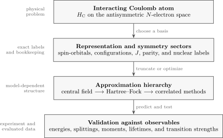
A reliable atomic-structure calculation separates the physical Hamiltonian from its representation and approximation. Configurations and orbitals help organize the problem; measured energies and transition properties test whether the chosen truncation is adequate.

The Multi-Electron Hamiltonian

For a nucleus of charge $+Ze$ fixed at the origin and $N$ nonrelativistic electrons, the Coulomb Hamiltonian in atomic units is

$$\begin{aligned} H_{\mathrm C} ={}&\sum_{i=1}^{N} \left( -\frac{1}{2}\nabla_i^2 -\frac{Z}{r_i} \right)\\ &+\sum_{i<j}\frac{1}{r_{ij}}, \qquad r_{ij}=|\mathbf r_i-\mathbf r_j|. \end{aligned}$$

Atomic units set $\hbar=m_e=e=4\pi\epsilon_0=1$. The first sum contains one-electron kinetic energies and nuclear attractions. The second sum is the pairwise Coulomb repulsion. For $N=1$, the problem is hydrogenic and separable. For $N>1$, the variables $r_{ij}$ depend on two electron coordinates and prevent decomposition into independent one-electron eigenproblems.

The Hamiltonian alone is not the complete specification. Because electrons are spin-$1/2$ fermions, the total electronic wavefunction obeys

$$P_{ij}\Psi=-\Psi,$$

where $P_{ij}$ exchanges the complete spatial and spin coordinates in slots $i$ and $j$. More generally, for a permutation $\pi$,

$$P_{\pi}\Psi=\operatorname{sgn}(\pi)\Psi.$$

Thus the physical Hilbert space is the antisymmetric subspace of the $N$-fold one-electron space. Electron labels in a coordinate wavefunction are argument slots, not experimentally distinguishable identities.

Corrections and the declared Hamiltonian

At finer resolution one adds finite-nuclear-mass, relativistic, nuclear-structure, radiative, and external-field terms. A useful bookkeeping form is

$$\begin{aligned} H_{\mathrm{atom}} ={}&H_{\mathrm C} +\delta H_{\mathrm{recoil}} +\delta H_{\mathrm{rel}}\\ &+H_{\mathrm{hfs}} +H_{\mathrm{ext}} +\delta H_{\mathrm{rad}} +\cdots . \end{aligned}$$

The labels that remain exact depend on this declared Hamiltonian. The spin-independent Coulomb Hamiltonian commutes separately with $L^2$, $S^2$, and their projections. A rotationally invariant spin–orbit interaction generally preserves $J^2$ for $\mathbf J=\mathbf L+\mathbf S$ but not $L^2$ and $S^2$ separately. An external field may preserve only the projection along a selected axis. Statements about “good quantum numbers” are therefore always statements about an interaction hierarchy.

Why Exact Solutions Are Rare

Three obstacles reinforce one another.

Coordinate coupling

If electron–electron repulsion were removed, a product of one-electron orbitals could diagonalize the Hamiltonian. The term $1/r_{ij}$ couples the motion of every pair. Even helium depends on the three scalar distances $r_1$, $r_2$, and $r_{12}$; a product $\phi(r_1)\phi(r_2)$ cannot reproduce arbitrary dependence on $r_{12}$.

Fermionic antisymmetry

A generic product is not an admissible electron state. Antisymmetrizing it produces a determinant and already correlates exchange-related amplitudes. The determinant solves the kinematic exchange requirement exactly, but a single determinant does not generally solve dynamical electron avoidance.

Rapidly growing representation spaces

Suppose $M$ orthonormal spin-orbitals are retained. The number of $N$-electron determinants is

$$\dim\mathcal H_{N,M}=\binom{M}{N}.$$

Symmetry adaptation can reduce the matrix to sectors of fixed parity and angular momentum, but the combinatorial growth remains. Increasing the orbital basis, opening more shells for excitation, or including relativistic spinors can quickly make direct diagonalization impractical.

Nuclear-charge scaling

Rescale electron coordinates by $\boldsymbol\rho_i=Z\mathbf r_i$. The fixed-nucleus Hamiltonian becomes

$$\begin{aligned} \frac{H_{\mathrm C}}{Z^2} ={}& \sum_i \left( -\frac{1}{2}\nabla_{\rho_i}^2 -\frac{1}{\rho_i} \right)\\ &+\frac{1}{Z} \sum_{i<j}\frac{1}{\rho_{ij}}. \end{aligned}$$

This form explains why electron–electron repulsion is relatively weaker along a highly charged isoelectronic sequence: nuclear binding scales as $Z^2$, while the scaled pair interaction enters at relative order $1/Z$. It does not make neutral heavy atoms weakly correlated, because their electron number grows with $Z$, inner and outer shells occupy very different scales, and near-degeneracies can defeat naive power counting.

Pauli Principle and Shell Structure

A one-electron spin-orbital is a function

$$\chi_a(x)=\phi_a(\mathbf r)\eta_a(\sigma),$$

where $x=(\mathbf r,\sigma)$ combines spatial and spin coordinates. A determinant built from occupied spin-orbitals $\chi_{a_1},\ldots,\chi_{a_N}$ is

$$\Phi(x_1,\ldots,x_N) =\frac{1}{\sqrt{N!}} \det[\chi_{a_p}(x_q)].$$

If two columns correspond to the same spin-orbital, the determinant vanishes. That algebraic fact is Pauli exclusion. In a central-field basis, a subshell with orbital angular momentum $\ell$ contains

$$g_{\ell}=2(2\ell+1)$$

spin-orbitals: $2\ell+1$ values of $m_\ell$ and two spin projections. Summing over $\ell=0,1,\ldots,n-1$ gives the hydrogenic shell capacity

$$\sum_{\ell=0}^{n-1}2(2\ell+1)=2n^2.$$

These capacities are exact counting statements for the chosen one-electron basis. The energetic order in which subshells fill is not fixed by Pauli exclusion. It depends on screening, penetration, exchange, relativistic shifts, and correlation. This is why the Aufbau mnemonic is useful but not an exact theorem about neutral-atom ground states.

Configurations are basis descriptions

A notation such as

$$1s^2\,2s^2\,2p^2$$

specifies occupation numbers of selected subshells. It does not by itself specify a unique antisymmetric state: the open $2p^2$ subshell supports several determinants, terms, and levels. Nor must an exact eigenstate have one configuration. In a configuration-interaction description,

$$|\Psi_{\Gamma}\rangle =\sum_I c_I|\Phi_{I\Gamma}\rangle,$$

where all basis functions share the exact symmetry label $\Gamma$, such as total $J$ and parity. A reported “leading configuration” identifies the largest component in a declared basis and coupling convention. It is not an observable probability independent of orbital choices.

Approximation Hierarchy

No single method is “the atomic approximation.” Each level answers a different question and omits a different class of effects.

Description	Trial space or variable	Captures	Characteristic omission
central field	one-electron orbitals in $V_{\mathrm{eff}}(r)$	shells, penetration, approximate quantum defects	explicit configuration mixing and pair correlation
Hartree	product orbitals and a direct self-consistent field	average Coulomb screening	fermionic antisymmetry in its raw product form
Hartree–Fock	one optimized determinant	antisymmetry, direct and exchange fields	correlation beyond one determinant
multiconfiguration or CI	linear combination of determinants or symmetry-adapted functions	configuration mixing and selected correlation	omitted excitations and orbital-space truncation
many-body perturbation theory	corrections about a reference state	systematic classes of virtual excitations when convergent	sensitivity to small denominators and reference choice
coupled cluster	exponential excitation ansatz	size-consistent correlation hierarchy	truncation cost and multireference difficulty
density-functional methods	electron density and approximate functionals	efficient ground-state energetics and densities	functional error and state-specific spectroscopy challenges
quantum Monte Carlo	stochastic many-electron sampling	flexible explicit correlation	statistical and fixed-node or phase errors

This table compares organizing ideas, not universal accuracy rankings. A carefully converged CI calculation for a few-electron atom and a density-functional calculation for a heavy open-shell atom answer different computational questions.

Central-field orbitals

The central-field starting point replaces the coupled problem by one-electron equations

$$\left[ -\frac{1}{2}\nabla^2 +V_{\mathrm{eff}}(r) \right]\phi_{n\ell m}(\mathbf r) =\varepsilon_{n\ell}\phi_{n\ell m}(\mathbf r).$$

Spherical symmetry supplies $n$, $\ell$, $m_\ell$, and parity labels. The effective potential includes the nuclear attraction and an averaged screening contribution. The resulting orbitals are useful coordinates for the many-electron problem; their eigenvalues are generally not the exact removal or excitation energies of the atom.

Hartree and Hartree–Fock

Hartree Method develops the self-consistent atomic direct field, radial equations, self-exclusion, and energy bookkeeping. For electrons, an antisymmetric mean-field state is instead a Slater determinant. Its energy can be written schematically as

$$E_{\mathrm{HF}} =\sum_a h_{aa} +\frac{1}{2}\sum_{a,b} \left(J_{ab}-K_{ab}\right),$$

where $a,b$ run over occupied spin-orbitals. The direct and exchange integrals are

$$J_{ab} ={} \iint |\chi_a(x)|^2 \frac{|\chi_b(x')|^2}{|\mathbf r-\mathbf r'|} \,dx\,dx'.$$ $$\begin{aligned} K_{ab} ={}&\iint \chi_a^*(x)\chi_b(x) \\ &\times \frac{\chi_b^*(x')\chi_a(x')} {|\mathbf r-\mathbf r'|} \,dx\,dx'. \end{aligned}$$

The $J$ term is the classical-looking Coulomb average. The $K$ term arises from antisymmetry and has no interpretation as an additional classical force. Variation under orbital orthonormality constraints gives self-consistent Fock equations. In a canonical orbital basis,

$$F\chi_a=\varepsilon_a\chi_a.$$

The equations are nonlinear because $F$ depends on the occupied orbitals. Convergence of an iterative solver proves only that a fixed point was found; one must still test energy stationarity, symmetry, numerical resolution, and possible lower-energy solutions.

Hartree–Fock for Atoms develops the atomic specialization: spherical closed shells, open-shell averaging choices, radial direct and exchange multipoles, occupied-orbital asymptotics, Koopmans-style ionization, and radial-grid versus orbital-basis diagnostics.

Exchange and Correlation

The words exchange and correlation are related but should not be merged. Exchange follows from fermionic antisymmetry and is already present in a single determinant. In conventional electronic-structure language, correlation is the residual pair response that the best determinant cannot represent.

Exchange and Correlation is the canonical atomic treatment. It derives direct and crossed Coulomb matrix elements, fixed-orbital singlet–triplet splitting, exchange- and correlation-hole sum rules, dynamical versus static correlation, and the distinct bookkeeping used by Hartree–Fock and density-functional theory.

Angular-Momentum Coupling

For a rotationally invariant nonrelativistic atom, define

$$\begin{gathered} \mathbf L=\sum_i\mathbf l_i, \qquad \mathbf S=\sum_i\mathbf s_i,\\ \mathbf J=\mathbf L+\mathbf S. \end{gathered}$$

If residual electrostatic interactions establish $L$ and $S$ before spin–orbit coupling resolves $J$, Russell–Saunders or $LS$ coupling is useful. Levels are labeled

$${}^{2S+1}L_J,$$

with parity supplied separately. The electronic parity of a configuration is

$$\pi=(-1)^{\sum_i\ell_i}.$$

For heavier atoms, one-electron spin–orbit interactions can be strong enough that each

$$\mathbf j_i=\mathbf l_i+\mathbf s_i$$

is coupled first, followed by

$$\mathbf J=\sum_i\mathbf j_i.$$

This is the $jj$ coupling limit. Most real open-shell atoms lie somewhere between ideal limits. Intermediate-coupling eigenstates are linear combinations of basis states with the same exact $J$ and parity. A term label can remain useful as a dominant-component name, but its purity should not be assumed.

Energy-scale criterion

Let $\Delta E_{\mathrm{el}}$ denote a representative residual electrostatic term separation and $\zeta$ a spin–orbit scale. Then

$$\begin{array}{ccl} \zeta\ll\Delta E_{\mathrm{el}} &:& LS,\\ \zeta\gg\Delta E_{\mathrm{el}} &:& jj,\\ \zeta\sim\Delta E_{\mathrm{el}} &:& \text{intermediate coupling}. \end{array}$$

The first two rows indicate the corresponding useful limiting basis. This is a diagnostic, not a sharp phase boundary. Near-degenerate levels of the same $J$ and parity can mix strongly even when the atom is otherwise well described by $LS$ coupling.

Spectroscopic Consequences

Atomic-structure models are tested by observables, not by the visual plausibility of orbitals. For two stationary levels $u$ and $l$,

$$\hbar\omega_{ul}=E_u-E_l, \qquad \lambda_{ul}=\frac{2\pi c}{\omega_{ul}}.$$

Level energies probe the Hamiltonian and correlation treatment. Fine- and hyperfine-structure intervals probe smaller relativistic and nuclear couplings. Landé factors and Zeeman patterns test angular-momentum composition. Transition amplitudes test both initial- and final-state wavefunctions; a calculation can reproduce energies while still predicting poor line strengths.

For an electric-dipole transition, the reduced line strength is conventionally built from

$$S_{ul} =\left| \langle \gamma_uJ_u \|D^{(1)}\| \gamma_lJ_l\rangle \right|^2,$$

where $\gamma$ collects additional state labels. Selection rules determine when symmetry forces this matrix element to vanish, while configuration mixing determines whether nominally weak channels borrow amplitude. The canonical derivation of these rules belongs to Atomic Selection Rules.

Oscillator Strengths owns the conversion from this reduced line strength to level-averaged $f$, $gf$, and Einstein $A$ values, including the required transition-energy and degeneracy factors.

Reading evaluated data carefully

The NIST Atomic Spectra Database reports critically evaluated energy levels, wavelengths, transition probabilities where available, ground states, and ionization energies. Its fields distinguish observed values, Ritz values derived from optimized level differences, uncertainties, and levels inferred by interpolation or theory. A database label should be read with its uncertainty and provenance rather than treated as exact notation.

When comparing calculation and data, record at least:

1. isotope and ionization stage;
2. zero of energy and unit convention;
3. Hamiltonian terms included;
4. basis and correlation truncation;
5. relativistic and finite-nuclear-size treatment;
6. whether a wavelength is observed or Ritz-derived;
7. uncertainty and source of each benchmark value.

Agreement with one transition does not validate the entire wavefunction. A trustworthy benchmark set spans absolute or relative energies, splittings, $g$ factors, lifetimes, branching ratios, and matrix elements sensitive to different regions of the state.

Chapter Sequence

The chapter develops the subject in the following order. Titles without links are forthcoming pages and are intentionally not linked until their routes exist.

Page	Central question
Multi-Electron Atoms	What structure organizes the interacting atomic problem?
Helium Atom	What already changes in the first genuinely interacting atom?
Electron Configurations	What does an occupation label say, and what does it omit?
Pauli Principle in Atoms	How does antisymmetry constrain atomic shell states?
Exchange and Correlation	Which effects arise from antisymmetry, and which lie beyond mean field?
Hartree Method	How is an average direct field determined self-consistently?
Hartree–Fock for Atoms	How does an antisymmetric mean field organize atomic orbitals and energies?
Slater Determinants in Atoms	How do determinants, configurations, and configuration-state functions differ?
LS Coupling	When are $L$, $S$, and $J$ useful atomic labels?
jj Coupling	How does strong one-electron spin–orbit coupling reorganize the basis?
Hund’s Rules	Why do familiar ordering rules work, and where do they fail?
Periodic Table from Quantum Mechanics	How do exclusion, screening, and shell energetics produce periodic trends?
Atomic Correlation Methods Overview	Which post-mean-field method matches a given atom and observable?

Suggested reading paths

First encounter: begin with Helium Atom, Electron Configurations, Pauli Principle in Atoms, and Exchange and Correlation. Then read the two mean-field pages, Slater Determinants in Atoms, LS Coupling, and jj Coupling.

Spectroscopy: review Atomic Term Symbols, then follow LS Coupling, jj Coupling, Hund’s Rules, and Atomic Selection Rules.

Electronic structure: review the Variational Principle, then follow Hartree Method, Hartree–Fock for Atoms, Slater Determinants in Atoms, and Atomic Correlation Methods Overview. The full generic derivations remain in the many-body volume.

Periodic trends: begin with Central-Field Approximation and Atomic Orbitals Revisited, then read Electron Configurations, Pauli Principle in Atoms, Hund’s Rules, and Periodic Table from Quantum Mechanics.

A Reliability Checklist

Before accepting a multi-electron atomic calculation, ask:

• Hamiltonian: Are recoil, relativistic, QED, nuclear-size, and external-field terms included at the resolution claimed?
• Symmetry: Which quantum numbers are exact for that Hamiltonian, and which are only dominant-component labels?
• Reference: Is one determinant qualitatively adequate, or are near-degenerate configurations essential?
• Basis: Are radial extent, angular functions, continuum-like orbitals, and core excitations converged for the target observable?
• Correlation: Which excitation classes or functional approximations are omitted?
• Numerics: Was the self-consistent solution checked for stability and against alternative initial guesses?
• Uncertainty: Are basis, truncation, constants, nuclear inputs, and experimental uncertainties separated?
• Validation: Are several observables compared with critically evaluated data?

This checklist is more informative than attaching a method name to a result. “Hartree–Fock,” “CI,” or “coupled cluster” identifies a family; reproducibility requires the Hamiltonian, basis, truncation, and convergence criteria.

Common Mistakes

Treating orbitals as observable electron paths

An orbital is a one-electron function used to represent a many-electron state. Rotations among occupied Hartree–Fock orbitals leave the determinant unchanged up to phase. Orbital pictures are useful, but individual electrons do not carry persistent orbital identities.

Attributing shell order to Pauli exclusion alone

Pauli exclusion sets occupancy constraints. The relative energies of $4s$, $3d$, and other subshells depend on the self-consistent potential, configuration, ionization state, and correlation.

Calling every same-spin effect exchange

Exchange follows from antisymmetry and is present in a determinant. Correlation describes missing many-electron structure relative to a declared reference. Neither term should be used as a vague synonym for electron repulsion.

Interpreting Hartree–Fock orbital energies as an exact spectrum

Koopmans-style relations use frozen orbitals and omit relaxation and correlation. Excitation energies generally require energy differences or response/state-specific methods, not raw orbital-energy spacings.

Assuming a configuration or term label is exact

Configuration weights depend on the orbital basis. $LS$ term labels become approximate under spin–orbit and configuration mixing. Exact labels should be tied to commuting symmetries such as total $J$ and parity for an isolated rotationally invariant atom.

Comparing numbers from different Hamiltonians

A nonrelativistic clamped-nucleus energy, a finite-mass value, and a relativistic/QED value are different theoretical quantities. Their numerical differences are not automatically “correlation energy.”

Exercises

Exercise 1: Nuclear-charge scaling

Starting from the atomic-unit Coulomb Hamiltonian, verify the $Z$-scaled form and identify the relative order of electron–electron repulsion along a fixed-$N$ isoelectronic sequence.

Solution

Set $\boldsymbol\rho_i=Z\mathbf r_i$. Then $\nabla_{r_i}=Z\nabla_{\rho_i}$, $r_i=\rho_i/Z$, and $r_{ij}=\rho_{ij}/Z$. Therefore

$$-\frac{1}{2}\nabla_{r_i}^2 -\frac{Z}{r_i} =Z^2 \left( -\frac{1}{2}\nabla_{\rho_i}^2 -\frac{1}{\rho_i} \right),$$

while

$$\frac{1}{r_{ij}}=\frac{Z}{\rho_{ij}} =Z^2\frac{1}{Z\rho_{ij}}.$$

Factoring out $Z^2$ gives a pair interaction of relative order $1/Z$. This argument holds at fixed electron number; it does not by itself control the neutral-atom limit $N=Z$.

Exercise 2: Subshell capacities

Find the maximum occupations of $s$, $p$, $d$, and $f$ subshells. Then verify that a hydrogenic shell with principal quantum number $n$ contains $2n^2$ spin-orbitals.

Solution

For a given $\ell$, there are $2\ell+1$ values of $m_\ell$ and two spin projections, so

$$g_{\ell}=2(2\ell+1).$$

Thus the capacities are $2$, $6$, $10$, and $14$ for $s$, $p$, $d$, and $f$. In shell $n$, the allowed values are $\ell=0,\ldots,n-1$, so

$$\begin{aligned} g_n &=2\sum_{\ell=0}^{n-1}(2\ell+1)\\ &=2n^2. \end{aligned}$$

The result counts basis states; it does not predict their energy ordering in a many-electron atom.

Exercise 3: Helium spin and spatial symmetry

For two electrons, the spin singlet is antisymmetric and the three triplet spin states are symmetric. What symmetry must the spatial factor have in each case? Which class can have nonzero amplitude at $\mathbf r_1=\mathbf r_2$?

Solution

The total electron state must be antisymmetric. Therefore a singlet spin factor must multiply a symmetric spatial factor, while a triplet spin factor must multiply an antisymmetric spatial factor:

$$\begin{array}{c|cc} &\text{spin}&\text{space}\\ \hline S=0&-&+\\ S=1&+&- \end{array}$$

Here $+$ denotes symmetry and $-$ denotes antisymmetry under electron exchange.

At coincident coordinates, antisymmetry gives

$$\psi_{\mathrm{space}}(\mathbf r,\mathbf r) =-\psi_{\mathrm{space}}(\mathbf r,\mathbf r)=0.$$

Hence a triplet spatial state vanishes at coincidence. A singlet spatial state is not forced to vanish there, although Coulomb correlation still modifies its short-range behavior.

Exercise 4: Finite-basis correlation energy

In one orbital basis, a Hartree–Fock calculation gives $E_{\mathrm{HF}}=-2.84\,E_{\mathrm h}$ and full configuration interaction gives $E_{\mathrm{FCI}}=-2.89\,E_{\mathrm h}$. Compute the finite-basis correlation energy. Why should it not be compared directly with a relativistic experimental binding energy?

Solution

Using the consistent finite-basis definition,

$$\begin{aligned} E_{\mathrm{corr}}^{(\mathcal B)} &=E_{\mathrm{FCI}}^{(\mathcal B)} -E_{\mathrm{HF}}^{(\mathcal B)}\\ &=-2.89\,E_{\mathrm h} -(-2.84\,E_{\mathrm h})\\ &=-0.05\,E_{\mathrm h}. \end{aligned}$$

Both values describe the same nonrelativistic Hamiltonian in the same orbital basis. An experimental binding energy also contains finite-mass, relativistic, radiative, and nuclear-structure contributions and uses an experimental energy zero. Subtracting unlike quantities would mix correlation with changes of Hamiltonian and convention.

Exercise 5: Choosing a coupling scheme

Consider two open-shell atoms. In atom A, residual electrostatic term separations are much larger than one-electron spin–orbit splittings. In atom B, the order is reversed. Which limiting coupling scheme is better for each, and which labels remain safest in intermediate coupling?

Solution

Atom A is closer to the $LS$ limit: first couple the orbital angular momenta to $L$ and spins to $S$, then couple $L$ and $S$ to $J$. Atom B is closer to the $jj$ limit: first form each $j_i=l_i\pm1/2$, then couple the $j_i$ values to total $J$.

In intermediate coupling, $L$, $S$, and the individual $j_i$ values may be basis labels rather than exact quantum numbers. For an isolated rotationally and parity-invariant atom, total $J$ and parity remain the safest exact electronic labels.

Exercise 6: Configuration mixing

An eigenstate with fixed $J$ and parity is written in an orthonormal configuration-state basis as

$$\begin{aligned} |\Psi\rangle ={}&\sqrt{0.70}\,|\Phi_1\rangle\\ &-\sqrt{0.25}\,|\Phi_2\rangle\\ &+\sqrt{0.05}\,|\Phi_3\rangle. \end{aligned}$$

What can be inferred from these coefficients, and why is “the atom is in configuration 1 with probability $70\%$” too strong without qualification?

Solution

Within this declared orthonormal basis, $\Phi_1$ is the leading component and its squared coefficient is $0.70$. The relative sign also matters for interference in matrix elements. However, configuration weights change when the orbital basis is rotated or reoptimized, and configurations are generally not projective observables measured independently of that representation. A careful statement is: “configuration-state function $\Phi_1$ carries $70\%$ weight in the specified expansion.” Total $J$, parity, and predictions for observables have a basis-independent physical meaning.

Cross-Links

• Common Atomic Hamiltonians gives the compact Coulomb operator, correction ledger, and model-boundary checks used throughout this chapter.
• Oscillator Strength Reference converts reduced atomic line strengths into $f$, $gf$, $\log(gf)$, and $A$ with explicit level weights.
• Atomic, Molecular, and Optical Physics
• Atomic Physics
• Helium Atom
• Electron Configurations
• Pauli Principle in Atoms
• Exchange and Correlation
• Hartree Method
• Hartree–Fock for Atoms
• Slater Determinants in Atoms
• LS Coupling
• jj Coupling
• Hund’s Rules
• Periodic Table from Quantum Mechanics
• Atomic Correlation Methods Overview
• Central-Field Approximation
• Atomic Orbitals Revisited
• Atomic Term Symbols
• Atomic Selection Rules
• Identical Particles and Exchange Symmetry
• Spin and Spatial Wavefunctions
• Pauli Exclusion Principle
• Slater Determinants
• Hartree Approximation
• Hartree–Fock Approximation
• Mean-Field Theory
• Angular Momentum Coupling Schemes
• Oscillator Strengths
• Variational Estimate for the Helium Atom
• AMO Physics Roadmap

References

1. W. C. Martin and W. L. Wiese, “Atomic Spectroscopy: An Introduction”, in G. W. F. Drake, ed., Atomic, Molecular, and Optical Physics Handbook, AIP Press, 1996; NIST online revision, accessed 2026-07-21.
2. A. Kramida, Yu. Ralchenko, J. Reader, and the NIST ASD Team, NIST Atomic Spectra Database, version 5.12, National Institute of Standards and Technology, 2024, DOI: 10.18434/T4W30F, accessed 2026-07-21.
3. R. D. Cowan, The Theory of Atomic Structure and Spectra, University of California Press, 1981.
4. W. R. Johnson, Atomic Structure Theory: Lectures on Atomic Physics, Springer, 2007.
5. B. H. Bransden and C. J. Joachain, Physics of Atoms and Molecules, 2nd ed., Pearson, 2003.
6. H. A. Bethe and E. E. Salpeter, Quantum Mechanics of One- and Two-Electron Atoms, Springer, 1957.
7. E. U. Condon and G. H. Shortley, The Theory of Atomic Spectra, Cambridge University Press, 1935.
8. C. Froese Fischer, T. Brage, and P. Jönsson, Computational Atomic Structure: An MCHF Approach, Institute of Physics Publishing, 1997.
9. P.-O. Löwdin, “Correlation Problem in Many-Electron Quantum Mechanics. I. Review of Different Approaches and Discussion of Some Current Ideas,” Advances in Chemical Physics 2, 207–322 (1959), DOI: 10.1002/9780470143599.ch2.
10. A. Szabo and N. S. Ostlund, Modern Quantum Chemistry: Introduction to Advanced Electronic Structure Theory, Dover, 1996.
11. I. P. Grant, Relativistic Quantum Theory of Atoms and Molecules: Theory and Computation, Springer, 2007.