Hartree Approximation

The Hartree approximation minimizes the expectation value of an interacting many-particle Hamiltonian over uncorrelated product states. Each particle moves in a one-body potential generated by the probability densities of all the others, so the one-body equations and the fields appearing in them must be solved self-consistently.

For distinguishable particles, the trial state has the form

$$\Psi_{\mathrm H}(q_1,\ldots,q_N) = \prod_{i=1}^{N}\phi_i(q_i).$$

For identical bosons in a simple condensate, every factor is the same normalized orbital. A raw product of labeled orbitals is not an admissible state of identical fermions; antisymmetry leads instead to a Slater-determinant variational family and exchange terms.

Hartree theory is therefore more specific than the general instruction to replace fluctuations by averages. It is a restricted variational theory with a precisely stated trial manifold. That precision gives it three important properties:

• the optimized energy is an upper bound when the product is an admissible trial state;
• the direct potential and its double-counting correction follow from one energy functional;
• every omitted effect can be traced to structure absent from the product manifold, especially exchange and connected interparticle correlations.

Canonical Scope

This page is the canonical home for:

• the Hartree product ansatz for distinguishable particles and simple bosonic condensates;
• the product-state energy functional and its constrained variation;
• direct self-consistent potentials and orbital equations;
• pair counting, the bosonic $N-1$ factor, and interaction double counting;
• the Coulomb Hartree potential, Poisson form, and self-interaction bookkeeping;
• a correlated two-oscillator benchmark that can be solved exactly;
• static and time-dependent Hartree formulations;
• controlled mean-field limits, diagnostics, and characteristic failures.

Other pages retain their own canonical material. General product states and entanglement are developed in Product States. The exact variational upper-bound theorem belongs to the Variational Principle. Hartree Method owns the spherical atomic specialization, self-excluded ionic tail, coupled radial equations, and atomic SCF diagnostics. The screened-charge calculation for helium remains in Helium Atom Variational Estimate. Fermionic determinants and exchange begin with Slater Determinants, while dilute-gas physics beyond a direct static shift is previewed in Weakly Interacting Bose Gas.

Hamiltonian and Assumptions

Consider a first-quantized Hamiltonian

$$H = \sum_{i=1}^{N}h_i + \frac{1}{2} \sum_{i\ne j}v_{ij}.$$

Here $q_i$ denotes all one-particle coordinates needed for particle $i$, possibly including position and internal labels. The one-body operator $h_i$ contains kinetic energy and external fields. For the main derivation, assume that the interaction is a real, symmetric, local pair potential,

$$v_{ij} = v_{ji}, \qquad v_{ij}(q,q') = v_{ji}(q',q).$$

The factor $1/2$ prevents counting an unordered pair twice. Equivalently,

$$\frac{1}{2} \sum_{i\ne j}v_{ij} = \sum_{i<j}v_{ij}.$$

This convention must remain fixed throughout a calculation. Many apparent factors-of-two disagreements in Hartree formulas come from switching silently between ordered and unordered pair sums.

The same variational logic extends to nonlocal pair kernels. The effective Hartree operator may then be nonlocal rather than multiplication by a function, but it is still obtained by contracting one particle line with the one-body state of another particle.

Product-State Trial Manifold

For distinguishable particles, choose independently normalized orbitals,

$$\langle\phi_i|\phi_i\rangle = 1, \qquad i=1,\ldots,N,$$

and form

$$|\Psi_{\mathrm H}\rangle = |\phi_1\rangle \otimes\cdots\otimes |\phi_N\rangle.$$

No orthogonality condition is required. The factors live in different labeled one-particle Hilbert spaces, so an overlap such as $\langle\phi_i|\phi_j\rangle$ need not even be defined when the species differ.

For a simple condensate of $N$ identical bosons, the state is instead

$$|\Psi_{\mathrm H}^{(B)}\rangle = |\phi\rangle^{\otimes N}, \qquad \langle\phi|\phi\rangle=1.$$

Because every factor is identical, this state is already symmetric. More general bosonic mean-field families can use several orbitals and symmetrized permanents, but they describe fragmentation and introduce additional occupation and orthogonality structure. They are not the elementary Hartree ansatz considered here.

What factorization asserts

For operators $A_i$ and $B_j$ acting on different factors,

$$\langle A_iB_j\rangle_{\mathrm H} = \langle A_i\rangle_{\mathrm H} \langle B_j\rangle_{\mathrm H}, \qquad i\ne j.$$

Thus every connected cross-particle correlator vanishes:

$$\langle A_iB_j\rangle_{\mathrm H,c} \equiv \langle A_iB_j\rangle_{\mathrm H} - \langle A_i\rangle_{\mathrm H} \langle B_j\rangle_{\mathrm H} =0.$$

The orbitals may be strongly distorted by the average interaction field, so Hartree theory is not generally a weak perturbation of the noninteracting orbitals. What remains absent is joint dependence on two or more coordinates beyond the product.

Hartree Energy Functional

The one-body contribution factorizes immediately:

$$\langle\Psi_{\mathrm H}|h_i|\Psi_{\mathrm H}\rangle = \langle\phi_i|h_i|\phi_i\rangle.$$

Define the direct pair integral

$$J_{ij} = \int dq\,dq'\, |\phi_i(q)|^2 v_{ij}(q,q') |\phi_j(q')|^2.$$

For a symmetric interaction, $J_{ij}=J_{ji}$. The product-state energy is

$$\begin{aligned} E_{\mathrm H}[\{\phi_i\}] ={}& \sum_i \langle\phi_i|h_i|\phi_i\rangle \\ &+ \frac{1}{2} \sum_{i\ne j}J_{ij}. \end{aligned}$$

In coordinate form,

$$\begin{aligned} E_{\mathrm H} ={}& \sum_i \int dq\, \phi_i^*(q)h_i\phi_i(q) \\ &+ \frac{1}{2} \sum_{i\ne j} \int dq\,dq'\, |\phi_i(q)|^2 v_{ij}(q,q') |\phi_j(q')|^2. \end{aligned}$$

The interaction energy depends on the full set of orbital densities. Consequently, varying one orbital changes both its own kinetic and external energy and every pair term containing that orbital.

Constrained Variational Derivation

Minimize $E_{\mathrm H}$ subject to independent normalization constraints. Introduce real Lagrange multipliers $\epsilon_i$ and the functional

$$\mathcal L = E_{\mathrm H} - \sum_i \epsilon_i \left( \langle\phi_i|\phi_i\rangle-1 \right).$$

Treat $\phi_i$ and $\phi_i^*$ as independent variables during variation. The one-body term gives

$$\frac{\delta}{\delta\phi_i^*(q)} \langle\phi_i|h_i|\phi_i\rangle = h_i\phi_i(q).$$

Particle $i$ appears in both ordered versions of each pair integral. The prefactor $1/2$ cancels that duplication:

$$\begin{aligned} \frac{\delta}{\delta\phi_i^*(q)} \left[ \frac{1}{2} \sum_{k\ne l}J_{kl} \right] ={}& \sum_{j\ne i} \left[ \int dq'\, |\phi_j(q')|^2 v_{ij}(q,q') \right] \phi_i(q). \end{aligned}$$

This identifies the direct Hartree potential seen by particle $i$:

$$V_i^{\mathrm H}(q) = \sum_{j\ne i} \int dq'\, |\phi_j(q')|^2 v_{ij}(q,q').$$

Stationarity, $\delta\mathcal L/\delta\phi_i^*=0$, gives the coupled Hartree equations

$$\left[ h_i+V_i^{\mathrm H}[\{\phi_j\}] \right] \phi_i = \epsilon_i\phi_i.$$

The notation emphasizes that $V_i^{\mathrm H}$ is a functional of all the other orbitals. The equation is linear in $\phi_i$ when the other orbitals are held fixed, but the full system is nonlinear.

Physical interpretation

The quantity $|\phi_j(q')|^2dq'$ is the probability of finding particle $j$ near $q'$. Hartree theory replaces the pair interaction with particle $j$ by its average over this distribution:

$$v_{ij}(q,q_j) \longrightarrow \int dq'\, |\phi_j(q')|^2v_{ij}(q,q').$$

Particle $i$ then moves in the external field plus the sum of these averaged fields. Its new orbital changes its density, which changes the fields seen by the other particles. A Hartree solution is a fixed point of this feedback loop.

Self-Consistency and Stationarity

A standard static iteration is:

1. choose normalized initial orbitals $\{\phi_i^{(0)}\}$;
2. construct every $V_i^{\mathrm H}$ from the current densities;
3. solve the effective one-body eigenproblems;
4. select the desired orbitals and normalize them;
5. mix old and new densities or orbitals if necessary;
6. repeat until densities, energy, and residuals converge.

An orbital residual is

$$R_i = \left( h_i+V_i^{\mathrm H}-\epsilon_i \right) \phi_i.$$

Small energy changes alone are not enough: cancellation can make the total energy appear stationary while one or more orbital equations remain inaccurate. A reliable calculation monitors norms such as $\|R_i\|$, density changes, interaction-energy consistency, and the original variational functional.

Convergence of the iteration establishes only a stationary point. Different seeds can converge to different local minima, excited self-consistent solutions, or symmetry-related branches. Restricted variation guarantees an upper bound for the global minimum in the trial family, not for an arbitrary converged fixed point interpreted as a ground-state estimate.

Meaning of the Orbital Multipliers

Multiplying the $i$th Hartree equation by $\phi_i^*$ and integrating gives

$$\epsilon_i = \langle\phi_i|h_i|\phi_i\rangle + \sum_{j\ne i}J_{ij}.$$

The multiplier $\epsilon_i$ enforces normalization and labels an effective one-body eigenvalue. It is not generally a literal share of the total energy. Summing over $i$ counts every pair interaction twice:

$$\sum_i\epsilon_i = \sum_i \langle\phi_i|h_i|\phi_i\rangle + \sum_{i\ne j}J_{ij}.$$

Therefore

$$E_{\mathrm H} = \sum_i\epsilon_i - \frac{1}{2} \sum_{i\ne j}J_{ij}.$$

The subtraction is the direct-interaction double-counting correction. Simply adding the occupied Hartree eigenvalues overestimates the variational energy.

Distinguishable Particles and Mixtures

The labeled-orbital derivation applies directly to distinguishable particles. It also generalizes naturally to mixtures in which each bosonic species occupies one orbital.

Let species $a$ contain $N_a$ particles in a normalized orbital $\phi_a$. Define

$$U_{ab} = \int dq\,dq'\, |\phi_a(q)|^2 v_{ab}(q,q') |\phi_b(q')|^2.$$

Then

$$\begin{aligned} E_{\mathrm H} ={}& \sum_a N_a \langle\phi_a|h_a|\phi_a\rangle \\ &+ \frac{1}{2} \sum_a N_a(N_a-1)U_{aa} \\ &+ \sum_{a<b}N_aN_bU_{ab}. \end{aligned}$$

Variation with respect to $\phi_a^*$ gives

$$\begin{aligned} \bigg[ h_a &+ (N_a-1)V_{aa}^{\mathrm H} \\ &+ \sum_{b\ne a}N_bV_{ab}^{\mathrm H} \bigg]\phi_a = \mu_a\phi_a, \end{aligned}$$

where

$$V_{ab}^{\mathrm H}(q) = \int dq'\, |\phi_b(q')|^2v_{ab}(q,q').$$

The same-species coefficient is $N_a-1$ because a particle does not interact with itself. The other-species coefficient is $N_b$ because all particles of species $b$ are genuine partners.

Identical Bosons in One Orbital

For $N$ identical bosons with the same one-body operator $h$ and symmetric pair potential $v$, use

$$\Psi_{\mathrm H}^{(B)}(q_1,\ldots,q_N) = \prod_{i=1}^{N}\phi(q_i).$$

There are $N$ one-body terms and $N(N-1)/2$ unordered pairs. Define

$$U[\phi] = \int dq\,dq'\, |\phi(q)|^2 v(q,q') |\phi(q')|^2.$$

The energy functional is

$$E_{\mathrm H}^{(B)}[\phi] = N\langle\phi|h|\phi\rangle + \frac{N(N-1)}{2}U[\phi].$$

Varying under $\langle\phi|\phi\rangle=1$ gives

$$\left[ h + (N-1)V_{\phi}^{\mathrm H}(q) \right] \phi(q) = \mu_{\mathrm H}\phi(q),$$

with

$$V_{\phi}^{\mathrm H}(q) = \int dq'\, |\phi(q')|^2v(q,q').$$

The factor $N-1$, rather than $N$, is exact within this finite-$N$ product ansatz. It encodes self-exclusion at the level of particle counting, even though the state has no correlation hole.

Multiplying the orbital equation by $\phi^*$ gives

$$\mu_{\mathrm H} = \langle h\rangle_\phi + (N-1)U[\phi].$$

By contrast, the energy per particle is

$$\frac{E_{\mathrm H}^{(B)}}{N} = \langle h\rangle_\phi + \frac{N-1}{2}U[\phi].$$

Thus the nonlinear orbital eigenvalue is not the energy per particle. Their interaction terms differ by a factor of two because adding one particle changes its interaction with every particle already present.

Contact Interaction and the Gross–Pitaevskii Boundary

If the effective pair interaction is modeled as

$$v(\mathbf r,\mathbf r') = g\,\delta^{(3)}(\mathbf r-\mathbf r'),$$

then

$$U[\phi] = g\int d^3r\,|\phi(\mathbf r)|^4,$$

and the bosonic Hartree equation becomes

$$\left[ h + g(N-1)|\phi(\mathbf r)|^2 \right] \phi(\mathbf r) = \mu_{\mathrm H}\phi(\mathbf r).$$

Writing a condensate wavefunction $\Phi=\sqrt{N}\phi$ gives

$$\left[ h + g\left(1-\frac{1}{N}\right)|\Phi|^2 \right] \Phi = \mu_{\mathrm H}\Phi.$$

At large $N$, this has the familiar form of the stationary Gross–Pitaevskii equation. The conceptual relation is close, but the theories should not be identified carelessly:

• elementary Hartree variation averages a specified pair potential over a product state;
• Gross–Pitaevskii theory uses a low-energy coupling fixed by the two-body scattering length;
• in the microscopic dilute-gas limit, short-range pair correlations can be essential even when the leading energy and density are described by a one-field functional;
• condensate depletion and Bogoliubov quasiparticles lie outside the pure product ansatz.

The focused Gross–Pitaevskii Equation treatment therefore owns the scattering-length matching, healing length, vortices, and condensate dynamics.

Why Raw Hartree Is Not a Fermion Theory

For identical fermions, a physical wavefunction must satisfy

$$\Psi(\ldots,q_i,\ldots,q_j,\ldots) = - \Psi(\ldots,q_j,\ldots,q_i,\ldots).$$

A labeled product

$$\phi_1(q_1)\phi_2(q_2)\cdots\phi_N(q_N)$$

does not have this transformation law. It is therefore not an admissible variational state for identical fermions, even if the orbitals are orthogonal.

Replacing the product by a Slater determinant restores antisymmetry. Evaluation of a two-body interaction in that determinant produces both direct and exchange integrals. The resulting Hartree–Fock equations are not merely Hartree equations supplemented by an optional empirical correction: exchange follows from the allowed fermionic trial manifold.

This distinction also clarifies terminology. In electronic-structure contexts, the phrase “Hartree term” often means only the direct density-generated contribution inside Hartree–Fock, density-functional, or Green-function equations. That direct term is meaningful, but a direct-only product theory is not by itself a valid many-electron wavefunction approximation.

Coulomb Hartree Potential

For particles with repulsive Coulomb interaction,

$$v(\mathbf r,\mathbf r') = \frac{e^2}{4\pi\epsilon_0} \frac{1}{|\mathbf r-\mathbf r'|},$$

an orbital density $n_j(\mathbf r)=|\phi_j(\mathbf r)|^2$ generates

$$V_{ij}^{\mathrm H}(\mathbf r) = \frac{e^2}{4\pi\epsilon_0} \int d^3r'\, \frac{n_j(\mathbf r')} {|\mathbf r-\mathbf r'|}.$$

The field seen by particle $i$ is the sum over $j\ne i$. If

$$n(\mathbf r) = \sum_j n_j(\mathbf r),$$

then a common total-density potential is

$$V_{\mathrm H}[n](\mathbf r) = \frac{e^2}{4\pi\epsilon_0} \int d^3r'\, \frac{n(\mathbf r')} {|\mathbf r-\mathbf r'|}.$$

It satisfies

$$\nabla^2V_{\mathrm H}[n](\mathbf r) = -\frac{e^2}{\epsilon_0}n(\mathbf r).$$

This sign corresponds to the positive potential energy of repulsion between two electrons. It should not be confused with the electrostatic scalar potential produced by negative charge, whose sign is opposite before multiplication by the test electron charge.

Self-interaction bookkeeping

The exact labeled Hartree equation uses $j\ne i$. Replacing that sum by the total density makes orbital $i$ feel its own density unless one subtracts

$$V_{ii}^{\mathrm H}(\mathbf r) = \frac{e^2}{4\pi\epsilon_0} \int d^3r'\, \frac{|\phi_i(\mathbf r')|^2} {|\mathbf r-\mathbf r'|}.$$

For one particle, any nonzero Coulomb Hartree field generated by its own density is manifestly spurious. In a finite bosonic condensate, the analogous correction is the difference between $N$ and $N-1$. In Hartree–Fock, exchange cancels the direct self-interaction of an occupied spin-orbital exactly, although correlation and approximate density functionals raise separate self-interaction questions.

Worked Benchmark: Two Coupled Oscillators

An exactly soluble model isolates what orbital relaxation can and cannot accomplish. Consider two distinguishable particles of equal mass in one-dimensional traps,

$$\begin{aligned} H ={}& \sum_{i=1}^{2} \left( \frac{p_i^2}{2m} + \frac{m\omega^2x_i^2}{2} \right) \\ &+ \frac{\kappa}{2}(x_1-x_2)^2, \qquad \kappa\ge 0. \end{aligned}$$

The interaction favors correlated displacements $x_1\simeq x_2$.

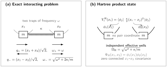
The exact Hamiltonian separates into center-of-mass and relative normal modes. Hartree variation replaces the coupling spring by two self-consistent one-body wells of frequency $\Omega_{\mathrm H}$; the optimized widths respond to $\kappa$, but a product state still has no connected $x_1$–$x_2$ covariance.

Exact solution

Introduce orthonormal normal coordinates

$$q_+ = \frac{x_1+x_2}{\sqrt{2}}, \qquad q_- = \frac{x_1-x_2}{\sqrt{2}}.$$

The normal-mode frequencies are

$$\omega_+ = \omega, \qquad \omega_- = \sqrt{\omega^2+\frac{2\kappa}{m}}.$$

Hence the exact ground-state energy is

$$E_0 = \frac{\hbar}{2} \left( \omega + \sqrt{\omega^2+\frac{2\kappa}{m}} \right).$$

The exact state is Gaussian in $q_+$ and $q_-$, but their unequal widths make it nonfactorizable in $x_1$ and $x_2$. In particular,

$$\langle x_1x_2\rangle_0 = \frac{\hbar}{4m} \left( \frac{1}{\omega} - \frac{1}{\omega_-} \right) >0$$

for $\kappa>0$.

Hartree minimization

By exchange symmetry of the Hamiltonian, use identical zero-centered Gaussian factors with a variational frequency $\Omega$,

$$\Psi_{\mathrm H}(x_1,x_2) = \phi_{\Omega}(x_1) \phi_{\Omega}(x_2).$$

For one factor,

$$\langle x^2\rangle_{\Omega} = \frac{\hbar}{2m\Omega}, \qquad \left\langle\frac{p^2}{2m}\right\rangle_{\Omega} = \frac{\hbar\Omega}{4}.$$

Factorization gives $\langle x_1x_2\rangle_{\mathrm H}=0$. The variational energy is

$$E_{\mathrm H}(\Omega) = \frac{\hbar}{2} \left[ \Omega + \frac{\omega^2+\kappa/m}{\Omega} \right].$$

Stationarity yields

$$\Omega_{\mathrm H} = \sqrt{\omega^2+\frac{\kappa}{m}}, \qquad E_{\mathrm H} = \hbar\Omega_{\mathrm H}.$$

The self-consistent field correctly narrows each one-particle orbital. Nevertheless,

$$E_{\mathrm H} - E_0 \ge 0,$$

with equality only for $\kappa=0$. Defining $\lambda=\kappa/(m\omega^2)$ gives the weak-coupling difference

$$E_{\mathrm H}-E_0 = \frac{\hbar\omega}{8}\lambda^2 + O(\lambda^3).$$

Hartree theory is correct through first order here because first-order perturbation theory needs only the unperturbed product density. The first missing energy appears at second order, where virtual correlated motion matters.

Density-Matrix View

For a distinguishable product state, the reduced state of particle $i$ is pure:

$$\rho_i^{(1)} = |\phi_i\rangle\langle\phi_i|.$$

For the simple $N$-boson product, two common one-body density-matrix conventions are

$$\gamma^{(1)} = |\phi\rangle\langle\phi|, \qquad \operatorname{Tr}\gamma^{(1)}=1,$$

or

$$\Gamma^{(1)} = N|\phi\rangle\langle\phi|, \qquad \operatorname{Tr}\Gamma^{(1)}=N.$$

The normalized two-body reduced state is also a product,

$$\gamma^{(2)} = |\phi\phi\rangle \langle\phi\phi|.$$

Mean-field convergence theorems are often stated as convergence of fixed-order reduced density matrices toward such tensor powers as $N\to\infty$. This is more precise than claiming that the full $N$-body wavefunction becomes close in norm: small correlations distributed across many particles can leave fixed-particle observables asymptotically factorized without making the entire many-body vector a literal product.

Time-Dependent Hartree Theory

Apply the Dirac–Frenkel variational principle to the time-dependent product manifold. Up to time-dependent orbital phase conventions, the distinguishable-particle equations are

$$i\hbar\frac{\partial}{\partial t}\phi_i(q,t) = \left[ h_i(t)+V_i^{\mathrm H}(q,t) \right] \phi_i(q,t),$$

where

$$V_i^{\mathrm H}(q,t) = \sum_{j\ne i} \int dq'\, |\phi_j(q',t)|^2 v_{ij}(q,q';t).$$

For $N$ identical bosons in one orbital,

$$i\hbar\partial_t\phi = \left[ h(t) + (N-1)V_{\phi}^{\mathrm H}(t) \right] \phi.$$

If $h$ and $v$ are time independent and the propagation is exact within the Hartree equations, norms and the Hartree energy are conserved. Independent transformations

$$\phi_i(t) \longrightarrow e^{i\theta_i(t)}\phi_i(t)$$

alter only scalar gauge terms in the orbital equations and multiply the total product by a global phase. Implementations may choose a gauge that removes orbital expectation values from the generators or improves numerical conditioning.

Time-dependent Hartree can describe collective changes in one-body densities, but it cannot generate entanglement from an initially factorized state because the trajectory is constrained to remain on the product manifold.

Mean-Field Scaling and Controlled Limits

For $N$ bosons in one orbital with an unscaled pair interaction, the interaction energy grows as $N^2$. A standard mean-field or Kac scaling uses

$$H_N = \sum_{i=1}^{N}h_i + \frac{1}{N-1} \sum_{i<j}v_{ij}.$$

The Hartree energy per particle is then

$$\frac{E_{\mathrm H}}{N} = \langle\phi|h|\phi\rangle + \frac{1}{2}U[\phi],$$

which remains finite as $N\to\infty$. The stationary equation becomes

$$\left[ h+V_{\phi}^{\mathrm H} \right]\phi = \mu\phi.$$

Under appropriate assumptions on the interaction, initial data, and observables, the many-body dynamics in this scaling converges to time-dependent Hartree dynamics at the level of reduced density matrices. The scaling and hypotheses are part of the theorem; “large $N$” by itself is not a proof that Hartree theory applies.

Other routes to mean-field accuracy include sufficiently long-range weak interactions, high connectivity with suitable coupling rescaling, or observables insensitive to short-distance correlations. The dilute Gross–Pitaevskii limit is different: it retains nontrivial two-body scattering correlations at short range while producing a nonlinear one-field description at leading order.

What Hartree Theory Captures

Within its domain, Hartree theory can capture:

• nonperturbative deformation of one-particle orbitals by average interactions;
• screening or broadening caused by smooth direct density fields;
• inhomogeneous density profiles in traps and external potentials;
• collective self-consistent motion in time-dependent fields;
• leading energies and fixed-particle observables in controlled mean-field limits;
• multiple stationary branches produced by nonlinear feedback.

The approximation is especially informative when the dominant interaction effect is a smooth field determined by many weak contributions and when connected few-body correlations are parametrically small for the observables of interest.

What the Product Manifold Omits

Exchange

Identical fermions require antisymmetry. Direct Hartree theory omits exchange energy, the exchange hole, and all consequences that follow from determinant structure.

Dynamical and static correlation

The product state cannot adjust the conditional position of one particle after another particle is observed. It misses correlation holes, pair cusps, correlated tunneling, dispersion forces between neutral fragments, and the coupled-oscillator covariance exhibited above.

Bosonic depletion and fragmentation

A single orbital has one macroscopically occupied natural orbital and zero depletion by construction. It cannot represent fragmented condensates or occupation of noncondensed modes.

Critical fluctuations

Near critical points, long-wavelength fluctuations may dominate and invalidate a smooth deterministic field even when a self-consistent solution exists.

Branch superpositions

Nonlinear Hartree equations can have symmetry-broken stationary solutions. The exact finite-system ground state may instead be a symmetric superposition of branches. A single product selects one branch and omits tunneling between them.

Short-range scattering structure

For singular or hard-core interactions, the exact wavefunction can develop rapid pair dependence at separations much shorter than the density-variation scale. Orbital optimization alone cannot build that pair structure.

Reliability Diagnostics

A Hartree result should be accompanied by checks that probe both the numerical solution and the trial manifold.

Numerical checks

• verify every orbital normalization;
• monitor orbital residuals, not only total-energy changes;
• compute the interaction energy both from pair integrals and from the fields;
• apply the double-counting correction when using orbital eigenvalues;
• repeat from symmetry-preserving and symmetry-breaking seeds;
• refine the basis, grid, and boundary conditions;
• for time evolution, monitor norm and conserved energy.

Physical checks

• recover the noninteracting limit continuously;
• verify the exact $N=1$ limit, including absence of self-interaction;
• compare with perturbation theory at weak coupling;
• test known symmetry and scaling properties;
• estimate connected correlations or compare with a richer ansatz;
• distinguish a mean-field large-$N$ limit from a dilute-gas or thermodynamic limit;
• benchmark small systems against exact diagonalization when feasible.

The product-state energy can be close while correlation-sensitive observables remain poor. Accuracy must be assessed observable by observable.

Common Mistakes

Treating self-consistency as exactness

A converged Hartree solution is exact only within the chosen product manifold. Iterating more tightly does not restore exchange or correlation.

Including the particle in its own field

The direct sum is $j\ne i$, and the bosonic coefficient is $N-1$. A total-density field without self-subtraction fails even the one-particle test.

Adding orbital eigenvalues to get the energy

The sum $\sum_i\epsilon_i$ counts each direct interaction twice. Use the variational functional or subtract half the ordered pair contribution.

Imposing unnecessary orthogonality

Labeled distinguishable-particle orbitals require normalization, not mutual orthogonality. Fermionic orthogonality belongs with determinant structure and exchange.

Calling a direct-only product a fermion wavefunction

Orthogonal orbitals do not make an unsymmetrized product antisymmetric. The trial state itself must obey particle statistics.

Replacing N − 1 by N Without Stating a Limit

The replacement may be harmless at leading order for large $N$, but it is not an exact finite-particle identity.

Identifying a bare contact potential with the physical coupling

In three dimensions, the low-energy coupling is tied to the scattering length. A naive delta potential and the renormalized Gross–Pitaevskii interaction are conceptually distinct steps.

Reporting only the lowest fixed point found

Nonlinear equations can have multiple branches. Seed dependence, Hessian information, and direct energy comparisons are part of identifying the relevant state.

Exercises

Derive the labeled Hartree equations

Starting from

$$E[\{\phi_i\}] = \sum_i\langle\phi_i|h_i|\phi_i\rangle + \frac{1}{2}\sum_{i\ne j}J_{ij},$$

vary with respect to $\phi_k^*$ and derive the orbital equation. Explain where the factor $1/2$ goes.

Solution

The constrained functional is

$$\mathcal L = E - \sum_i\epsilon_i \left( \langle\phi_i|\phi_i\rangle-1 \right).$$

The variation of the one-body term is $h_k\phi_k$. In the ordered pair sum, terms with $i=k$ and terms with $j=k$ both contribute. Symmetry of the pair potential makes the two contributions equal, so their sum cancels the prefactor $1/2$. Thus

$$\frac{\delta\mathcal L} {\delta\phi_k^*(q)} = \left[ h_k + \sum_{j\ne k} \int dq'\, |\phi_j(q')|^2v_{kj}(q,q') - \epsilon_k \right] \phi_k(q).$$

Setting this expression to zero gives

$$\left(h_k+V_k^{\mathrm H}\right) \phi_k = \epsilon_k\phi_k.$$

Recover the bosonic pair factors

For $N$ identical bosons in one normalized orbital, derive both the coefficient $N(N-1)/2$ in the energy and the coefficient $N-1$ in the orbital equation.

Solution

The number of unordered pairs chosen from $N$ particles is

$$\binom{N}{2} = \frac{N(N-1)}{2}.$$

Therefore

$$E[\phi] = N\langle h\rangle_\phi + \frac{N(N-1)}{2}U[\phi].$$

Both density factors in $U$ vary. Hence

$$\frac{\delta U}{\delta\phi^*(q)} = 2V_{\phi}^{\mathrm H}(q)\phi(q).$$

After dividing the stationary equation by the overall factor $N$, the interaction coefficient is

$$\frac{N(N-1)}{2} \frac{2}{N} = N-1.$$

Thus each boson feels the other $N-1$ bosons, not itself.

Correct the orbital-energy sum

Show that the total Hartree energy can be reconstructed from the orbital multipliers as

$$E_{\mathrm H} = \sum_i\epsilon_i - \frac{1}{2} \sum_{i\ne j}J_{ij}.$$

Solution

Taking the expectation value of each orbital equation gives

$$\epsilon_i = h_i^{(0)} + \sum_{j\ne i}J_{ij},$$

where $h_i^{(0)}=\langle\phi_i|h_i|\phi_i\rangle$. Summing gives

$$\sum_i\epsilon_i = \sum_i h_i^{(0)} + \sum_{i\ne j}J_{ij}.$$

The variational energy contains only half of the ordered pair sum. Subtracting the excess half yields the stated result.

Two bosonic species with contact interactions

Species $a$ and $b$ contain $N_a$ and $N_b$ bosons in normalized orbitals $\phi_a$ and $\phi_b$. Let

$$v_{aa}=g_{aa}\delta, \qquad v_{bb}=g_{bb}\delta, \qquad v_{ab}=g_{ab}\delta.$$

Derive the Hartree equation for species $a$.

Solution

The terms depending on $\phi_a$ are

$$\begin{aligned} E_a ={}& N_a\langle\phi_a|h_a|\phi_a\rangle \\ &+ \frac{g_{aa}}{2}N_a(N_a-1) \int dq\,|\phi_a|^4 \\ &+ g_{ab}N_aN_b \int dq\,|\phi_a|^2|\phi_b|^2. \end{aligned}$$

Variation and division by $N_a$ give

$$\left[ h_a + g_{aa}(N_a-1)|\phi_a|^2 + g_{ab}N_b|\phi_b|^2 \right] \phi_a = \mu_a\phi_a.$$

The same-species field excludes one $a$ boson; the cross-species field contains all $N_b$ particles.

Diagnose one-particle self-interaction

Suppose a Coulomb Hartree equation is written using the total density $n=|\phi|^2$ for a system with $N=1$. Show why the result is inconsistent and state the correction.

Solution

The total-density formula produces

$$V_{\mathrm H}(\mathbf r) = \frac{e^2}{4\pi\epsilon_0} \int d^3r'\, \frac{|\phi(\mathbf r')|^2} {|\mathbf r-\mathbf r'|},$$

which is nonzero for a normalized orbital. But the original pair Hamiltonian has no terms when $N=1$ because there is no pair. The exact Hartree sum $\sum_{j\ne i}$ is empty. One must therefore subtract the orbital’s own contribution or retain the explicit self-excluding sum from the start.

Mean-field scaling

For $N$ identical bosons, replace $v$ by $v/(N-1)$. Show that the Hartree energy per particle and orbital equation have finite, $N$-independent interaction terms.

Solution

The product-state energy is

$$E_{\mathrm H} = N\langle h\rangle + \frac{N(N-1)}{2} \frac{U}{N-1}.$$

Therefore

$$\frac{E_{\mathrm H}}{N} = \langle h\rangle + \frac{U}{2}.$$

The orbital equation contains the number of partners times the scaled interaction,

$$(N-1)\frac{V_{\phi}^{\mathrm H}}{N-1} = V_{\phi}^{\mathrm H}.$$

Hence

$$\left(h+V_{\phi}^{\mathrm H}\right)\phi = \mu\phi,$$

with no divergent coefficient as $N\to\infty$.

Minimize the coupled-oscillator product energy

For the two-oscillator benchmark, minimize

$$E_{\mathrm H}(\Omega) = \frac{\hbar}{2} \left[ \Omega + \frac{\omega^2+\kappa/m}{\Omega} \right]$$

and compare the weak-coupling expansion with the exact energy through order $\kappa^2$.

Solution

Differentiation gives

$$\frac{dE_{\mathrm H}}{d\Omega} = \frac{\hbar}{2} \left[ 1 - \frac{\omega^2+\kappa/m}{\Omega^2} \right].$$

The positive stationary point is

$$\Omega_{\mathrm H} = \sqrt{\omega^2+\frac{\kappa}{m}},$$

and it is a minimum. Set $\lambda=\kappa/(m\omega^2)$. Then

$$\frac{E_{\mathrm H}}{\hbar\omega} = \sqrt{1+\lambda} = 1+\frac{\lambda}{2} -\frac{\lambda^2}{8} +O(\lambda^3).$$

The exact result is

$$\begin{aligned} \frac{E_0}{\hbar\omega} &= \frac{1+\sqrt{1+2\lambda}}{2} \\ &= 1+\frac{\lambda}{2} -\frac{\lambda^2}{4} +O(\lambda^3). \end{aligned}$$

Thus

$$E_{\mathrm H}-E_0 = \frac{\hbar\omega}{8}\lambda^2 +O(\lambda^3).$$

Product states and connected covariance

Let $|\Psi\rangle=|\phi_1\rangle\otimes|\phi_2\rangle$. Prove that the connected covariance of $A_1$ and $B_2$ vanishes. Why can self-consistent orbital deformation not change this conclusion?

Solution

Tensor-product factorization gives

$$\begin{aligned} \langle\Psi|A_1B_2|\Psi\rangle ={}& \langle\phi_1|A_1|\phi_1\rangle \langle\phi_2|B_2|\phi_2\rangle. \end{aligned}$$

Therefore

$$\langle A_1B_2\rangle - \langle A_1\rangle\langle B_2\rangle =0.$$

Self-consistency changes $|\phi_1\rangle$ and $|\phi_2\rangle$, and therefore changes each one-body expectation value. It does not change the tensor-product form of the state, so the factorization identity remains exact everywhere on the Hartree manifold.

Key Takeaways

• Hartree theory is restricted variation over product states, not merely an informal replacement by averages.
• The direct field seen by one particle is the pair potential averaged over every other particle’s orbital density.
• The coupled orbital equations are nonlinear because their potentials depend on their own solution.
• The variational energy is not the sum of orbital eigenvalues; direct interactions require a double-counting subtraction.
• A finite simple bosonic condensate has $N(N-1)/2$ pairs and an $N-1$ orbital field.
• Raw labeled products are inadmissible for identical fermions; determinant antisymmetry generates exchange.
• Hartree orbital relaxation can be nonperturbative while connected interparticle correlations remain identically zero.
• Controlled mean-field limits require a specified scaling, hypotheses, and class of observables.
• Self-interaction, missing exchange, absent pair correlations, depletion, fragmentation, and critical fluctuations are central diagnostics.
• Exact small-system benchmarks reveal which errors arise from numerics and which arise from the product manifold itself.

Cross-Links

• Mean-Field Theory
• Interacting Many-Body Systems Overview
• First-Quantized Many-Body Wavefunctions
• Two-Body Operators
• Product States
• Slater Determinants
• Exchange and Correlation
• Hartree Method
• Variational Principle
• Helium Atom Variational Estimate
• Weakly Interacting Bose Gas Preview
• Correlation Functions Overview
• Normal Ordering in Many-Body QM
• Quantum Chemistry Roadmap

References

• D. R. Hartree, “The Wave Mechanics of an Atom with a Non-Coulomb Central Field. Part I. Theory and Methods,” Proceedings of the Cambridge Philosophical Society 24, 89–110 (1928), doi:10.1017/S0305004100011919.
• P. A. M. Dirac, “Note on Exchange Phenomena in the Thomas Atom,” Proceedings of the Cambridge Philosophical Society 26, 376–385 (1930), doi:10.1017/S0305004100016108.
• P. Pickl, “A Simple Derivation of Mean Field Limits for Quantum Systems,” Letters in Mathematical Physics 97, 151–164 (2011), doi:10.1007/s11005-011-0470-4.
• C. Bardos, L. Erdős, F. Golse, N. J. Mauser, and H.-T. Yau, “Derivation of the Schrödinger–Poisson Equation from the Quantum $N$-Body Problem,” Comptes Rendus Mathématique 334, 515–520 (2002), doi:10.1016/S1631-073X(02)02253-7.
• E. H. Lieb, R. Seiringer, and J. Yngvason, “Bosons in a Trap: A Rigorous Derivation of the Gross–Pitaevskii Energy Functional,” Physical Review A 61, 043602 (2000), doi:10.1103/PhysRevA.61.043602.
• H. Spohn, “Kinetic Equations from Hamiltonian Dynamics: Markovian Limits,” Reviews of Modern Physics 52, 569–615 (1980), doi:10.1103/RevModPhys.52.569.
• A. L. Fetter and J. D. Walecka, Quantum Theory of Many-Particle Systems, Dover (2003).
• J. W. Negele and H. Orland, Quantum Many-Particle Systems, Westview Press (1998).
• A. Szabo and N. S. Ostlund, Modern Quantum Chemistry: Introduction to Advanced Electronic Structure Theory, Dover (1996).
• P. Ring and P. Schuck, The Nuclear Many-Body Problem, Springer (1980), doi:10.1007/978-3-642-61852-9.
• L. Pitaevskii and S. Stringari, Bose–Einstein Condensation and Superfluidity, Oxford University Press (2016), doi:10.1093/acprof:oso/9780198758884.001.0001.
• J. Frenkel, Wave Mechanics: Advanced General Theory, Clarendon Press (1934).