Molecular Quantum Mechanics

A molecule is a quantum system of electrons and nuclei whose internal states can bind, rotate, vibrate, tunnel, dissociate, react, and exchange energy with radiation. Molecular structure is not inserted into the exact Coulomb Hamiltonian as a fixed arrangement of classical nuclei. It emerges through a hierarchy: separate overall translation, solve or approximate the coupled internal problem, exploit the electron–nuclear mass ratio, identify potential-energy surfaces, quantize nuclear motion, and connect transitions among the resulting rovibronic states to spectra and dynamics.

Three cautions organize the subject:

• Nuclei remain quantum particles. “Clamped nuclei” names an auxiliary electronic eigenproblem, not the final molecular model.
• Orbitals and structures are representations. The full observable state is a many-particle wavefunction or density operator with the required symmetries.
• Energy-scale separation is powerful but conditional. Near electronic degeneracies, avoided crossings, dissociation thresholds, and conical intersections, several electronic channels may have to be retained.

This chapter follows the path from the full molecular Hamiltonian to chemical and spectroscopic observables without treating a ball-and-stick picture as a microscopic premise.

Canonical Scope

This page is the chapter-level map for:

• the electronic, nuclear, spin, and rotational degrees of freedom of an isolated molecule;
• the distinction between the exact internal Hamiltonian and a clamped-nuclei electronic Hamiltonian;
• potential-energy surfaces, equilibrium geometries, barriers, and dissociation channels;
• molecular-orbital and valence-bond languages;
• rotational, vibrational, vibronic, and electronic states;
• molecular symmetry, identical-nucleus statistics, and spectroscopic labels;
• the route from energy levels and transition moments to spectra, thermochemistry, and reaction dynamics;
• where single-surface and fixed-structure pictures fail.

Born–Oppenheimer Approximation as Scale Separation owns the general derivation of electronic-channel equations, derivative couplings, small parameters, and validity tests. Born–Oppenheimer in Molecules owns equilibrium structures, isotope-dependent nuclear motion, rovibrational reductions, and molecular accuracy diagnostics. Potential Energy Surfaces owns landscape geometry, stationary points, reaction paths, crossings, computational representations, and uncertainty. Quantum Harmonic Oscillator and Rigid Rotor own the canonical model solutions. Molecular Rotation Applications owns the tensor-operator derivation of basic rotational selection rules. This page explains how those pieces fit into one molecular problem.

Nonadiabatic Coupling owns molecular transfer among electronic surfaces, surface-hopping logic, vibronic models, photochemical interpretation, and the handoff to geometric phase.

Conical Intersections owns degeneracy conditions, seam dimension, branching-plane geometry, MECIs, molecular Berry sign change, and conical-intersection validation.

What Makes Molecules Harder Than Atoms

An isolated atom already combines Coulomb interaction, fermionic antisymmetry, angular momentum, correlation, and relativity. A molecule adds several layers.

More dynamical particles

There are at least two nuclei, so internuclear distances and angles become quantum coordinates. Nuclear motion changes the electronic Hamiltonian, while the electronic state changes the forces governing nuclear motion.

No universal central field

Except for special limits, a molecule has no spherically symmetric one-center potential. Orbital angular momentum about one nucleus is generally not conserved. Point-group labels, body-fixed projections, total angular momentum, parity, and permutation symmetry replace the simple hydrogenic label set.

Several nested energy scales

Electronic excitation, vibration, rotation, tunneling, spin splittings, and hyperfine structure often occupy different energy ranges. Their hierarchy enables approximations but also produces dense spectra and many couplings.

Several physically relevant asymptotes

A molecular state can correlate with different separated-atom, ion-pair, or fragmentation channels. Binding must be defined relative to the correct threshold, including electronic terms, nuclear motion, and conserved quantum numbers.

Structure is an effective description

An exact stationary state of a freely rotating molecule respects the symmetries of the full Hamiltonian. A body-fixed equilibrium geometry is obtained from an effective potential surface and is extraordinarily useful, but it is not the same object as a sharply oriented laboratory-frame eigenstate.

The Laboratory-Frame Hamiltonian

Let $N_e$ electrons have coordinates $\mathbf r_i$, and let $N_N$ nuclei have coordinates $\mathbf R_A$, charges $Z_A$, and masses $M_A$. In Hartree atomic units, with nuclear masses expressed in electron-mass units, the nonrelativistic Coulomb Hamiltonian is

Molecular Hamiltonian gives the term-by-term operator ledger, exact symmetry analysis, center-of-mass derivation, finite-mass cross terms, and dissociation-threshold conventions. The compact form here is only the chapter-level starting point.

$$\begin{aligned} H_{\mathrm{lab}} ={}& -\frac12\sum_{i=1}^{N_e}\nabla_i^2 -\sum_{A=1}^{N_N} \frac{1}{2M_A}\nabla_A^2 \\ &+ \sum_{i<j}\frac{1}{r_{ij}} + \sum_{A<B}\frac{Z_AZ_B}{R_{AB}} \\ &- \sum_{i,A} \frac{Z_A}{ \lvert\mathbf r_i-\mathbf R_A\rvert }. \end{aligned}$$

Each term has a distinct role:

• the first line contains electronic and nuclear kinetic energy;
• the second line contains electron–electron and nucleus–nucleus repulsion;
• the third line contains electron–nucleus attraction.

There is no fundamental “bond potential” added to this Hamiltonian. Bonding, equilibrium geometry, barriers, and molecular spectra arise from its states and from controlled reductions of it.

This Hamiltonian omits relativistic interactions, coupling to external fields, finite nuclear size, radiative corrections, and nuclear internal excitations. Those terms can be added when the target uncertainty demands them.

Exchange symmetry is required twice

Electrons are identical fermions, so the total electronic state is antisymmetric under electron exchange. Identical nuclei must also obey their own bosonic or fermionic exchange symmetry, including nuclear spin. These are separate requirements:

$$P_{ij}^{(e)}\Psi=-\Psi,$$

while for identical nuclei $A$ and $B$,

$$P_{AB}^{(N)}\Psi = \begin{cases} +\Psi, & \text{bosonic nuclei},\\ -\Psi, & \text{fermionic nuclei}. \end{cases}$$

The electronic spatial-spin symmetry, nuclear-spin symmetry, rotation, and vibration must combine consistently. Ortho and para nuclear-spin isomers are a familiar consequence, not an optional spectroscopic correction.

Remove Overall Translation

For an isolated molecule with no external field, translational invariance implies conservation of total momentum. In atomic units, define

$$M_{\mathrm{tot}} = \sum_A M_A+N_e$$

and the center-of-mass coordinate

$$\mathbf R_{\mathrm{CM}} = \frac{ \sum_A M_A\mathbf R_A + \sum_i\mathbf r_i }{ M_{\mathrm{tot}} }.$$

A suitable change to center-of-mass and internal coordinates gives

$$H_{\mathrm{lab}} = -\frac{1}{2M_{\mathrm{tot}}} \nabla_{\mathrm{CM}}^2 + H_{\mathrm{int}}.$$

The wavefunction can be factored into a free center-of-mass state and an internal molecular state,

$$\Psi_{\mathrm{lab}} = e^{i\mathbf P\cdot\mathbf R_{\mathrm{CM}}/\hbar} \Psi_{\mathrm{int}}.$$

Exact internal coordinates can generate reduced-mass, mass-polarization, Coriolis, and other kinetic couplings. Their form depends on the coordinate convention; their physical predictions do not. Removing overall translation is exact for the isolated nonrelativistic problem, whereas separating electronic, vibrational, and rotational motion is generally approximate.

Electronic and Nuclear Degrees of Freedom

After translation is removed, it is useful to classify internal variables by what changes.

Sector	Typical coordinates or labels	Physical content
Electronic	electron positions, electronic spin, occupations, electronic symmetry	charge distribution, exchange, correlation, electronic excitation
Vibrational	bond stretches, bends, torsions, collective normal coordinates	shape fluctuations, zero-point motion, tunneling, dissociation
Rotational	orientation and body-fixed angular momentum	overall molecular rotation and rotational fine structure
Nuclear spin	nuclear-spin projections and coupled spin labels	exchange statistics and hyperfine structure
Coupled rovibronic	total angular momentum, parity, vibronic symmetry	observable stationary levels of the internal Hamiltonian

The separation among these sectors is a model organization. The exact internal Hamiltonian can couple all degrees of freedom allowed by symmetry.

Counting nuclear shape coordinates

For $N_N$ nuclei in three dimensions there are $3N_N$ Cartesian coordinates. Remove three overall translations. For a nonlinear equilibrium geometry, remove three rotations, leaving

$$N_{\mathrm{vib}} = 3N_N-6.$$

For a linear molecule, rotation about the molecular axis does not change the nuclear configuration, so only two rotational coordinates are removed:

$$N_{\mathrm{vib}}^{\mathrm{linear}} = 3N_N-5.$$

These counts describe small-amplitude vibrational coordinates near a nondegenerate equilibrium geometry. Floppy molecules, internal rotors, dissociation coordinates, and coordinate singularities may require a less local description.

Born–Oppenheimer Separation

Born–Oppenheimer in Molecules develops the molecular application in detail, including equilibrium structures, normal modes, isotope scaling, diagonal corrections, and the distinction between bare, adiabatic, and coupled-surface treatments.

The mass ratio

$$\frac{m_e}{M_A}\ll1$$

suggests organizing the internal problem into fast electronic and slow nuclear motion. At each nuclear geometry $R$, solve an electronic eigenproblem

$$H_e(R) \lvert\phi_\alpha(R)\rangle = E_\alpha(R) \lvert\phi_\alpha(R)\rangle.$$

There are two common conventions:

• include the internuclear repulsion $V_{NN}(R)$ in $H_e$, so $E_\alpha(R)$ is already a potential-energy surface;
• exclude $V_{NN}$ from $H_e$ and define

$$U_\alpha(R) = E_\alpha^{(e)}(R)+V_{NN}(R).$$

Both are valid when stated and used consistently.

An exact electronic-channel expansion is

$$\Psi(r,R) = \sum_\alpha \chi_\alpha(R) \phi_\alpha(r;R).$$

The leading one-surface approximation retains one channel and neglects off-diagonal derivative couplings:

$$\left[ T_N+U_\alpha(R) \right] \chi_{\alpha\nu}(R) = E_{\alpha\nu} \chi_{\alpha\nu}(R).$$

The electronic state has not disappeared. Its eigenvalue supplies the nuclear potential, and its geometry dependence controls the omitted couplings.

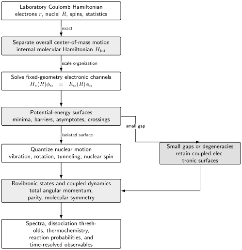
The molecular hierarchy. Overall translation separates exactly for an isolated molecule. The later electronic-surface and rovibrational reductions require scale, symmetry, and gap checks; small electronic gaps redirect the calculation to a coupled-surface description.

Where the approximation enters

The channel expansion itself is exact for a complete electronic basis. Approximation enters when channels are discarded or when nuclear derivatives of $\phi_\alpha(r;R)$ are neglected. For nondegenerate channels,

$$\mathbf d_{\alpha\beta}(R) = \langle\phi_\alpha| \nabla_R\phi_\beta\rangle_e$$

is related schematically to

$$\mathbf d_{\alpha\beta} \sim \frac{ \langle\phi_\alpha| \nabla_RH_e |\phi_\beta\rangle_e }{ E_\beta-E_\alpha }.$$

A small nuclear velocity does not compensate for a vanishing electronic gap. Avoided crossings and conical intersections can therefore invalidate a one-surface picture even when nuclei are heavy.

What “fast electrons” does not mean

The approximation is not based on assigning classical orbital periods to electrons and nuclei. It is a spectral and asymptotic statement about a slow–fast Hamiltonian, channel gaps, derivative couplings, nuclear momenta, and the region of configuration space occupied by the state.

Potential-Energy Surfaces

A potential-energy surface $U_\alpha(R)$ is an electronic eigenvalue, including internuclear repulsion under the convention used here, as a function of nuclear geometry. Translation and global rotation do not change it. Its independent dimensions are therefore usually $3N_N-6$ for a nonlinear molecule and $3N_N-5$ for a linear molecule. The dedicated Potential Energy Surfaces page develops coordinate metrics, stationary-point index, reaction paths, barriers, asymptotes, multistate crossings, and fit validation.

Minima and equilibrium geometry

An equilibrium geometry $R_e$ on one surface satisfies

$$\nabla_RU_\alpha(R_e)=0,$$

with a positive Hessian in the stable internal directions. The geometry $R_e$ is the minimum of an effective surface. It need not equal:

• the expectation value of a bond length in a vibrational state;
• a thermally averaged diffraction geometry;
• the most probable geometry in every coordinate measure;
• a structure that remains meaningful near dissociation or strong nonadiabatic mixing.

Nuclear zero-point motion samples a region around the minimum even at zero temperature.

Barriers, saddles, and reaction coordinates

A first-order saddle on a surface often organizes a reaction pathway: the Hessian has one unstable direction and stable directions transverse to it. The barrier height alone does not determine a rate. Zero-point energies, tunneling, entropy, recrossing, multiple pathways, solvent or environment, and coupling among surfaces can all matter.

Dissociation thresholds

For a diatomic ground-state surface with asymptote $U(\infty)$ and minimum $U(R_e)$, the well depth is

$$D_e = U(\infty)-U(R_e).$$

The dissociation energy from the lowest vibrational level is smaller:

$$D_0 = D_e-E_{\mathrm{ZP}},$$

when the separated fragments carry no corresponding vibrational zero-point contribution. Experimental threshold conventions must specify fragment electronic states, isotope, and internal excitation.

Surfaces are representation dependent near degeneracy

Adiabatic surfaces diagonalize $H_e(R)$ point by point. A diabatic representation trades diagonal electronic energies for smoother off-diagonal couplings. Individual surfaces and derivative couplings depend on that representation; the predictions of a consistently transformed coupled-channel calculation do not.

Bonding as a Quantum Phenomenon

A chemical bond is not represented by one unique Hermitian “bond operator.” Several complementary diagnostics answer different questions:

• a bound minimum relative to specified fragmentation thresholds;
• electron-density accumulation or depletion;
• reduced density matrices and pair densities;
• energy decomposition within a declared scheme;
• vibrational frequencies and force constants;
• dissociation energies and reaction energetics;
• localized orbitals, bond orders, or resonance weights defined within a representation.

Chemical Bonding owns the operational definition, the covalent–ionic–metallic and weak-interaction limits, and the hierarchy from observable evidence to representation-dependent analyses. The chapter summary below keeps only the route through those ideas.

Molecular-orbital language

Molecular Orbitals develops the one-electron language in detail. Molecular orbitals are often expanded in atom-centered basis functions,

$$\psi_p(\mathbf r) = \sum_\mu C_{\mu p}\chi_\mu(\mathbf r).$$

Bonding and antibonding labels describe phase and density patterns within a chosen one-electron model. Occupying orbitals produces an antisymmetrized many-electron reference, not the exact state automatically. Orbital energies, shapes, and localization depend on the approximation and orbital rotations allowed.

H₂⁺ Ion is the canonical worked bridge from this language to a molecular Hamiltonian and potential curve. Because H₂⁺ has only one electron, its exact fixed-center orbital, minimal LCAO approximation, nuclear repulsion, and two-state interpretation can be compared without electron-correlation ambiguities.

Hydrogen Molecule adds the smallest possible electron–electron problem. It compares Heitler–London, restricted molecular-orbital, broken-symmetry, and configuration-interaction descriptions against the same neutral-fragment dissociation test.

Electronic Structure Overview compares the fixed-geometry electronic equation, basis sets, Hartree–Fock, configuration interaction, coupled cluster, density-functional theory, multireference methods, excited-state routes, and validation. Detailed derivations stay in their canonical method pages.

Valence-bond language

Valence Bond Theory develops localized atomic-like orbitals, spin coupling, ionic and covalent structures, and resonance among them. These descriptions can expose local pairing and dissociation physics that a single delocalized determinant hides. Molecular-orbital and valence-bond expansions span the same exact Hilbert space when both are complete; practical truncations emphasize different structures.

Binding is a total-energy statement

For fragments $A$ and $B$, a molecular state is stable against that channel when

$$E_{AB} < E_A+E_B$$

for energies computed with the same Hamiltonian, masses, relativistic content, basis-limit convention, and fragment quantum numbers. Calling one orbital “bonding” is not a substitute for this comparison.

Exchange, electrostatics, kinetic-energy redistribution, polarization, and correlation are not independent fundamental forces. They are useful components of particular analyses of the same interacting quantum state.

Rotations and Vibrations

Near a stable minimum, nuclear motion can often be organized into normal vibrations and overall rotation.

Harmonic normal modes

Let $q_a$ be internal displacements from $R_e$. Expanding the surface gives

$$U(R) \approx U(R_e) + \frac12 \sum_{a,b} K_{ab}q_aq_b.$$

After mass weighting and diagonalizing the Hessian, one obtains normal coordinates $Q_k$ with

$$H_{\mathrm{vib}}^{(0)} = \sum_k \left[ -\frac{\hbar^2}{2} \frac{\partial^2}{\partial Q_k^2} + \frac12\omega_k^2Q_k^2 \right].$$

The harmonic energies are

$$E_{\mathrm{vib}}^{(0)} = \sum_k \hbar\omega_k \left( v_k+\frac12 \right).$$

Real molecular surfaces are anharmonic. Mode coupling, resonances, large-amplitude motion, torsion, tunneling, and dissociation eventually invalidate independent harmonic oscillators.

Normal Modes of Polyatomics owns the Cartesian generalized eigenproblem, rigid-motion projection, symmetry classification, infrared and Raman activity, and computational frequency diagnostics.

Overall rotation

For a rigid body with principal moments of inertia $I_a$, $I_b$, and $I_c$,

$$H_{\mathrm{rot}} = \frac{J_a^2}{2I_a} + \frac{J_b^2}{2I_b} + \frac{J_c^2}{2I_c}.$$

Linear, spherical-top, symmetric-top, and asymmetric-top molecules have different spectra. The diatomic limit reduces to

$$E_J = \frac{\hbar^2}{2I}J(J+1).$$

Vibration changes the moments of inertia, rotation stretches bonds, and body-fixed coordinates generate Coriolis couplings. Thus “rotation plus vibration” is a leading organization, not an exact additive decomposition.

Rotations of Molecules develops this applied rotor hierarchy, including rotational-constant conventions, isotope-sensitive inertia tensors, centrifugal distortion, polyatomic rotor classes, and microwave inference.

Vibrations of Diatomics applies the local oscillator to one molecular bond, distinguishes angular-frequency and spectroscopic-wavenumber conventions, develops anharmonic and Morse models, and connects dipole derivatives to infrared activity.

Rovibrational Coupling reunites these leading rotational and vibrational models into joint term values, P/Q/R branches, state-dependent rotational constants, Coriolis structure, line strengths, and a practical band-assignment workflow.

A typical spectroscopic hierarchy

For many stable molecules away from degeneracies,

$$\Delta E_{\mathrm{electronic}} \gg \Delta E_{\mathrm{vibrational}} \gg \Delta E_{\mathrm{rotational}}.$$

This is a useful empirical hierarchy, not a theorem. Floppy molecules, weak complexes, Rydberg states, near-degenerate electronic states, and large angular momentum can scramble it.

For a diatomic term expressed in wavenumbers, a common expansion is

$$\begin{aligned} \frac{E_{\alpha vJ}}{hc} \approx{}& T_\alpha +G_\alpha(v) +F_{\alpha v}(J), \\ G_\alpha(v) ={}& \omega_e \left(v+\frac12\right) -\omega_ex_e \left(v+\frac12\right)^2 +\cdots, \\ F_{\alpha v}(J) ={}& B_vJ(J+1) -D_v[J(J+1)]^2 +\cdots. \end{aligned}$$

The constants are fitted or computed effective parameters. They summarize the local spectrum; they are not a replacement for the underlying Hamiltonian outside their domain.

Electronic Excitations and Vibronic States

An electronic transition changes the electronic channel, but the nuclei do not disappear during the transition. Initial and final states have rovibrational structure on their respective surfaces.

Under a one-surface product approximation,

$$\Psi_i(r,R) \approx \phi_i(r;R)\chi_i(R), \qquad \Psi_f(r,R) \approx \phi_f(r;R)\chi_f(R).$$

For the electric-dipole operator, define the electronic transition dipole at fixed geometry,

$$\boldsymbol\mu_{fi}^{(e)}(R) = \langle\phi_f(R)| \widehat{\boldsymbol\mu} |\phi_i(R)\rangle_e.$$

The vibronic transition amplitude is then

$$\mathbf M_{fi} = \int \chi_f^*(R) \boldsymbol\mu_{fi}^{(e)}(R) \chi_i(R) \,dR.$$

In the Condon approximation, $\boldsymbol\mu_{fi}^{(e)}(R)$ is replaced by a nearly constant value over the nuclear wavepacket. Intensities then contain Franck–Condon overlaps,

$$\langle\chi_f|\chi_i\rangle.$$

The familiar “vertical transition” picture means that electronic excitation occurs on a time scale short compared with substantial nuclear displacement. It does not mean the nuclei have zero position uncertainty or that only one geometry contributes.

Vibronic coupling

Nuclear displacement can mix electronic states and can make otherwise forbidden transitions acquire intensity. Near a conical intersection, electronic and nuclear labels cannot be assigned independently over the whole relevant region. Geometric phase, nonadiabatic transfer, and ultrafast internal conversion are then central parts of the molecular dynamics.

Molecular Symmetry

Several symmetry groups appear, and they answer different questions.

Point groups at a geometry

The point group of a fixed nuclear framework classifies electronic orbitals, normal modes, and tensor components. Its irreducible representations predict which matrix elements vanish and how degeneracies are organized.

Molecular Symmetry develops the practical workflow from symmetry operations and character reduction to normal-mode, selection-rule, and orbital applications.

Full rotations and parity

An isolated field-free molecule is invariant under laboratory rotations. Total angular momentum and its space-fixed projection are therefore exact labels under the usual assumptions. Parity is exact when the Hamiltonian is inversion symmetric, even if a chosen equilibrium geometry is not itself centrosymmetric.

Permutation and inversion

Equivalent nuclei can be permuted through feasible or formal operations. Rovibronic and nuclear-spin functions must combine with the correct statistics. For nonrigid molecules, a molecular symmetry or permutation–inversion group can be more appropriate than the point group of one equilibrium geometry.

Symmetry labels do not guarantee purity

States with the same exact symmetry can mix. Conversely, approximate labels such as a dominant normal-mode occupation or electronic configuration can remain useful even when they are not conserved. A spectroscopic assignment should distinguish exact quantum numbers from approximate parentage.

From States to Spectra

The most basic spectral condition is

$$h\nu = E_f-E_i.$$

A line also requires a nonzero transition matrix element, an initial population, and a line-shape mechanism. Its observable strength depends on quantities such as

$$S_{fi} \propto |\langle f|\widehat O|i\rangle|^2,$$

with degeneracy, polarization, thermal population, and experimental geometry included as appropriate.

What different spectral regions probe

Spectral structure	Primary change and information
Microwave or rotational	Changes rotational quantum numbers and reveals moments of inertia, geometry, dipole moments, and hyperfine structure.
Infrared	Changes vibrational state, often with rotational branches, and probes force constants, anharmonicity, symmetry, and isotope shifts.
Raman	Uses polarizability-mediated rotation or vibration and supplies complementary symmetry and mode information.
Visible or ultraviolet	Changes electronic state with vibronic structure and probes excited surfaces, transition dipoles, and photodynamics.
Photoelectron	Removes an electron while resolving ionic rovibronic states, probing ionization energies, correlation signatures, and nuclear geometry change.

These are dominant associations, not exclusive categories. Fine, hyperfine, Zeeman, Stark, predissociation, collision, and environmental effects can appear across them.

Frequencies are not enough

A trustworthy interpretation also considers:

• transition selection rules and intensity borrowing;
• isotope dependence;
• temperature and state populations;
• natural, Doppler, collision, transit-time, and instrumental widths;
• unresolved hyperfine or rovibronic components;
• perturbations by nearby states;
• uncertainty and calibration of the measured line position.

Spectroscopy is an inverse problem: the Hamiltonian and assignments are inferred from finite, broadened data. A precise fit can still use an incomplete physical model.

Molecular Spectroscopy and Chemistry

Molecular quantum mechanics connects stationary structure to chemical change.

Thermochemistry

Partition functions sum rotational, vibrational, electronic, and nuclear-spin states. Zero-point energy and isotope dependence shift enthalpies and equilibrium constants. A consistent calculation must align energy zeros, degeneracies, symmetry numbers, and standard-state conventions.

Reaction dynamics

Potential surfaces organize trajectories and wavepacket propagation, but reaction probabilities require dynamics. Tunneling, resonances, nonadiabatic transitions, geometric phase, and interference can make a minimum-energy path an incomplete account.

Photochemistry

Light can prepare a nonequilibrium vibronic wavepacket on an excited surface. Its subsequent motion may fluoresce, internally convert, cross between spin manifolds, dissociate, or reach a conical intersection. The outcome depends on the prepared state and coupled dynamics, not only on a static orbital diagram.

Environments

Collisions, solvents, surfaces, cavities, and radiation fields broaden levels and exchange energy with the molecule. An isolated-molecule Hamiltonian is then a subsystem model. Open-system methods, condensed-phase coordinates, or quantized fields may be required.

How to Navigate This Chapter

The planned sequence follows the hierarchy of the problem:

1. state the full molecular Hamiltonian and separate overall translation;
2. apply Born–Oppenheimer reasoning to molecular structure;
3. interpret potential-energy surfaces, minima, barriers, and crossings;
4. compare molecular-orbital and valence-bond descriptions;
5. solve the one-electron molecular ion and the correlated hydrogen molecule;
6. develop chemical bonding without assigning one universal bond observable;
7. quantize molecular rotation, vibration, normal modes, and rovibrational coupling;
8. map electronic-structure methods and excited-state approximations;
9. treat nonadiabatic coupling and conical intersections;
10. use molecular symmetry to classify states, modes, and transitions.

Until the specialist pages are encountered, use Quantum Chemistry Roadmap for prerequisites and Quantum Chemistry References for reading routes.

Common Mistakes

“The nuclei are fixed in the Born–Oppenheimer approximation”

They are fixed only while solving the parameter-dependent electronic problem. Nuclear motion is then quantized on one or more electronic surfaces.

“A molecule has one exact geometry”

An equilibrium geometry is a minimum of an effective surface. A nuclear wavefunction has finite width, zero-point motion, rotational symmetry, and sometimes amplitude over several equivalent structures.

“A molecular orbital is the path of an electron”

An orbital is a basis-dependent one-electron function in an approximation. Electrons do not follow orbital-shaped trajectories.

“A bond is caused by exchange”

Exchange, electrostatics, kinetic energy, polarization, and correlation are components of a description. Stability is a total-state energy comparison against specified fragmentation channels.

“Every vibration is an independent harmonic oscillator”

Normal modes are a local quadratic approximation near a stable minimum. Anharmonicity, resonances, torsion, tunneling, and dissociation couple or replace them.

“Electronic, vibrational, and rotational labels are always exact”

They are approximate labels when coupling terms are present. Total angular momentum, parity, and exact molecular symmetry labels are usually safer, subject to the declared Hamiltonian.

“A spectral peak directly equals an energy level”

A peak is produced by a transition, population, matrix element, line shape, and instrument response. Blending and state mixing can complicate assignment.

Exercises

Exercise 1: Separate the center of mass

For particles with masses $m_a$, positions $\mathbf x_a$, and total momentum $\mathbf P=\sum_a\mathbf p_a$, explain why a translationally invariant Hamiltonian can be written as center-of-mass kinetic energy plus an internal Hamiltonian.

Solution

Define

$$M=\sum_a m_a, \qquad \mathbf R_{\mathrm{CM}} = \frac{1}{M} \sum_a m_a\mathbf x_a.$$

Choose $3(N-1)$ relative coordinates invariant under

$$\mathbf x_a\mapsto\mathbf x_a+\mathbf a.$$

Because the Coulomb potential depends only on coordinate differences, it is independent of $\mathbf R_{\mathrm{CM}}$. A canonical linear transformation of momenta decomposes the quadratic kinetic energy into

$$\sum_a\frac{\mathbf p_a^2}{2m_a} = \frac{\mathbf P^2}{2M} +T_{\mathrm{int}}.$$

Hence

$$H = \frac{\mathbf P^2}{2M} +H_{\mathrm{int}}.$$

The separation is exact for an isolated translation-invariant system. External fields can couple center-of-mass and internal motion, especially for charged systems in magnetic fields.

Exercise 2: Count vibrational modes

Find the number of small-amplitude vibrational modes of water, carbon dioxide, and methane. Treat water and methane as nonlinear and carbon dioxide as linear.

Solution

Water has $N_N=3$ nuclei and is nonlinear:

$$N_{\mathrm{vib}}(\mathrm{H_2O}) = 3(3)-6 =3.$$

Carbon dioxide also has three nuclei but is linear:

$$N_{\mathrm{vib}}(\mathrm{CO_2}) = 3(3)-5 =4.$$

The two perpendicular bending directions are degenerate in the linear equilibrium geometry but count as two normal coordinates.

Methane has $N_N=5$ nuclei and is nonlinear:

$$N_{\mathrm{vib}}(\mathrm{CH_4}) = 3(5)-6 =9.$$

Degeneracy groups frequencies into symmetry multiplets; it does not reduce the number of independent coordinates.

Exercise 3: Isotope scaling

In a diatomic molecule, hold the electronic potential curve fixed while changing isotopes. Show how the harmonic vibrational frequency and rigid-rotor constant scale with the nuclear reduced mass $\mu$.

Solution

Near equilibrium,

$$U(R) \approx U(R_e) + \frac12k(R-R_e)^2.$$

The harmonic frequency is

$$\omega_e = \sqrt{\frac{k}{\mu}},$$

so

$$\omega_e\propto\mu^{-1/2}.$$

The equilibrium moment of inertia is

$$I_e=\mu R_e^2.$$

The rotational constant in energy units is

$$B_e = \frac{\hbar^2}{2I_e} = \frac{\hbar^2}{2\mu R_e^2},$$

and therefore

$$B_e\propto\mu^{-1}.$$

The fixed-surface assumption is the leading Born–Oppenheimer isotope model. Adiabatic, nonadiabatic, and isotope-dependent structural corrections produce smaller deviations.

Exercise 4: Diagnose a failing one-surface model

Two electronic surfaces have a gap $\Delta E(R)$ that becomes very small in the region occupied by a nuclear wavepacket. The matrix element $\langle\phi_1|\nabla_RH_e|\phi_2\rangle$ remains finite. What happens to the derivative coupling, and what model should replace an isolated-surface calculation?

Solution

Away from exact degeneracy, the off-diagonal derivative coupling behaves schematically as

$$\mathbf d_{12} \sim \frac{ \langle\phi_1|\nabla_RH_e|\phi_2\rangle }{ \Delta E(R) }.$$

As $\Delta E$ becomes small, the coupling can become large. The electronic eigenvectors change rapidly with geometry, so a nuclear wavepacket cannot remain in one adiabatic channel merely because the nuclei are heavy.

One should retain at least the two relevant channels and solve coupled nuclear equations, possibly in a diabatic or locally smooth basis. Near a conical intersection, geometric-phase consistency must also be checked.

Exercise 5: Distinguish well depth and dissociation energy

A diatomic potential has minimum $0.20\,\mathrm{eV}$ below its separated-fragment asymptote. Its vibrational zero-point energy relative to the minimum is $0.03\,\mathrm{eV}$. Neglect fragment internal excitation. Find $D_e$ and $D_0$.

Solution

The well depth is measured from the potential minimum:

$$D_e = 0.20\,\mathrm{eV}.$$

The lowest vibrational state lies $0.03\,\mathrm{eV}$ above that minimum, so the energy required to dissociate from that state is

$$\begin{aligned} D_0 &=D_e-E_{\mathrm{ZP}}\\ &=0.20\,\mathrm{eV}-0.03\,\mathrm{eV}\\ &=0.17\,\mathrm{eV}. \end{aligned}$$

Reporting only “bond energy” would leave the reference ambiguous.

Exercise 6: Read the energy hierarchy

A spectrum contains spacings near $0.2\,\mathrm{meV}$, $0.15\,\mathrm{eV}$, and $3\,\mathrm{eV}$. Give a plausible leading assignment and one reason the assignment is not guaranteed from scale alone.

Solution

A common assignment is:

$$\begin{aligned} 0.2\,\mathrm{meV} &:\ \text{rotation},\\ 0.15\,\mathrm{eV} &:\ \text{vibration},\\ 3\,\mathrm{eV} &:\ \text{electronic excitation}. \end{aligned}$$

The hierarchy is plausible for a stable small molecule. It is not guaranteed because weak complexes can have very soft vibrations, fine or spin–orbit structure can lie in rotational or vibrational ranges, Rydberg electronic spacings can be small, and observed lines usually combine several quantum-number changes. Selection rules, isotope shifts, intensities, and detailed level patterns are needed.

Exercise 7: Franck–Condon overlap

In the Condon approximation, an electronic transition dipole is independent of $R$. Show how the vibronic amplitude factorizes and explain why a transition between two allowed electronic states can still have a weak vibrational line.

Solution

If

$$\boldsymbol\mu_{fi}^{(e)}(R) \approx \boldsymbol\mu_{fi}^{(e)}(R_0),$$

then

$$\begin{aligned} \mathbf M_{fi} &= \int \chi_f^*(R) \boldsymbol\mu_{fi}^{(e)}(R_0) \chi_i(R)\,dR \\ &= \boldsymbol\mu_{fi}^{(e)}(R_0) \langle\chi_f|\chi_i\rangle. \end{aligned}$$

The electronic factor may be nonzero while the nuclear overlap is small because the two surfaces have different equilibrium geometries, curvatures, or mode coordinates. The particular vibronic line is then weak even though the electronic transition is symmetry allowed. Intensity is distributed across the Franck–Condon progression.

Key Takeaways

• The exact nonrelativistic molecular Hamiltonian contains electronic and nuclear kinetic energy plus Coulomb interactions; a bond potential is not fundamental input.
• Overall translation separates exactly for an isolated molecule. Electronic, vibrational, and rotational separations require approximation and symmetry analysis.
• The Born–Oppenheimer method produces electronic potential-energy surfaces and quantum nuclear motion; it does not turn nuclei into fixed classical points.
• Equilibrium geometry is a surface minimum, while a molecular state includes zero-point motion, rotation, exchange symmetry, and sometimes tunneling among structures.
• Molecular-orbital and valence-bond descriptions are complementary representation languages, not competing microscopic realities.
• Rotational and vibrational models arise from moments of inertia and local surface curvature, with anharmonic, Coriolis, and nonadiabatic corrections.
• Spectra measure transitions with intensities and line shapes, not isolated energy levels directly.
• Near small electronic gaps and conical intersections, coupled-surface dynamics replaces the single-surface picture.

Cross-Links

• AMO Bibliography and Reading Guide routes among molecular symmetry, effective-Hamiltonian, spectroscopy, and electronic-structure sources.
• Atomic, Molecular, and Optical Physics
• Common Molecular Hamiltonians
• Atomic Physics
• Multi-Electron Atoms
• Atomic Correlation Methods Overview
• Born–Oppenheimer Approximation as Scale Separation
• Born–Oppenheimer in Molecules
• Potential Energy Surfaces
• Molecular Orbitals
• Electronic Structure Overview
• Nonadiabatic Coupling
• Conical Intersections
• Molecular Symmetry
• Valence Bond Theory
• H₂⁺ Ion
• Hydrogen Molecule
• Chemical Bonding
• Rotations of Molecules
• Vibrations of Diatomics
• Normal Modes of Polyatomics
• Rovibrational Coupling
• Cold Molecules
• Born–Oppenheimer Berry Phase
• Molecular Physics Application Map
• Quantum Harmonic Oscillator
• Oscillator as a Universal Local Model
• Rigid Rotor
• Rotational Spectra
• Molecular Rotation Applications
• Groups and Representations
• Identical Particles
• Quantum Chemistry Roadmap
• Quantum Chemistry References

References

1. M. Born and R. Oppenheimer, “Zur Quantentheorie der Molekeln,” Annalen der Physik 389, 457–484 (1927), doi:10.1002/andp.19273892002.
2. M. Born and K. Huang, Dynamical Theory of Crystal Lattices, Oxford University Press (1954), Appendix VIII.
3. H. C. Longuet-Higgins, “The Intersection of Potential Energy Surfaces in Polyatomic Molecules,” Proceedings of the Royal Society A 344, 147–156 (1975), doi:10.1098/rspa.1975.0095.
4. R. G. Woolley and B. T. Sutcliffe, “Molecular Structure and the Born–Oppenheimer Approximation,” Chemical Physics Letters 45, 393–398 (1977), doi:10.1016/0009-2614(77)80298-4.
5. W. Domcke and D. R. Yarkony, “Role of Conical Intersections in Molecular Spectroscopy and Photoinduced Chemical Dynamics,” Annual Review of Physical Chemistry 63, 325–352 (2012), doi:10.1146/annurev-physchem-032210-103522.
6. P. W. Atkins and R. S. Friedman, Molecular Quantum Mechanics, 5th ed., Oxford University Press (2011).
7. I. N. Levine, Quantum Chemistry, 7th ed., Pearson (2014).
8. D. A. McQuarrie, Quantum Chemistry, 2nd ed., University Science Books (2008).
9. G. Herzberg, Molecular Spectra and Molecular Structure I: Spectra of Diatomic Molecules, 2nd ed., Van Nostrand (1950).
10. G. Herzberg, Molecular Spectra and Molecular Structure II: Infrared and Raman Spectra of Polyatomic Molecules, Van Nostrand (1945).
11. G. Herzberg, Molecular Spectra and Molecular Structure III: Electronic Spectra and Electronic Structure of Polyatomic Molecules, Van Nostrand (1966).
12. P. R. Bunker and P. Jensen, Molecular Symmetry and Spectroscopy, 2nd ed., NRC Research Press (1998).
13. J. M. Brown and A. Carrington, Rotational Spectroscopy of Diatomic Molecules, Cambridge University Press (2003), doi:10.1017/CBO9780511814808.
14. E. B. Wilson Jr., J. C. Decius, and P. C. Cross, Molecular Vibrations: The Theory of Infrared and Raman Vibrational Spectra, Dover (1980).
15. T. Helgaker, P. Jørgensen, and J. Olsen, Molecular Electronic-Structure Theory, Wiley (2000), doi:10.1002/9781119019572.
16. NIST, Molecular Microwave Spectral Databases, Standard Reference Databases 114, 115, and 117, accessed 2026-07-21.
17. NIST, Chemistry WebBook Guide: Vibrational and Electronic Spectra and Constants of Diatomic Molecules, Standard Reference Database 69, accessed 2026-07-21.