Born–Oppenheimer Approximation as Scale Separation

The Born–Oppenheimer approximation uses the large disparity between nuclear and electronic masses to organize molecular quantum mechanics into fast electronic and slow nuclear problems. At each nuclear configuration, one first diagonalizes an electronic Hamiltonian. Its eigenvalues become potential-energy surfaces for the nuclear motion; derivatives of its eigenvectors couple those surfaces.

The slogan “electrons adjust instantaneously to fixed nuclei” captures the leading picture, but it hides the approximation’s actual content. The nuclei are not made classical, “fixed nuclei” describes only an auxiliary electronic eigenproblem, and a small mass ratio does not by itself guarantee single-surface dynamics. The decisive questions are whether the relevant electronic subspace remains spectrally isolated and whether nuclear motion can resolve the changing electronic eigenvectors.

This page owns the method: its scale hierarchy, exact electronic-channel equations, one-surface reduction, and practical validity tests. Molecular Hamiltonian owns the all-particle Coulomb operator, exact center-of-mass separation, and finite-mass coordinate terms. Born–Oppenheimer in Molecules owns the application to equilibrium structures, isotope-dependent nuclear motion, rovibrational states, and molecular spectroscopy. Potential Energy Surfaces owns stationary-point geometry, reaction paths, barriers, crossings, computational representations, and surface uncertainty. Molecular Quantum Mechanics owns the broader application hierarchy for bonding, electronic structure, reaction dynamics, and chemical interpretation. The Molecular Physics application map organizes the symmetry prerequisites, while Born–Oppenheimer Berry Phase owns the geometric phase and gauge structure.

Nonadiabatic Coupling owns the molecular dynamics built from several coupled surfaces: avoided-crossing passage, surface hopping, vibronic models, and photochemical interpretation.

Conical Intersections owns codimension-two seam geometry, branching-plane normal forms, MECIs, molecular Berry sign change, and computational diagnostics at exact degeneracy.

The Approximation in One Line

The construction is a sequence, not a single product ansatz:

$$\begin{gathered} H_{\mathrm{mol}} = T_N+H_e(R), \\ H_e(R)\lvert\phi_a(R)\rangle = E_a(R)\lvert\phi_a(R)\rangle, \\ \Psi(r,R) = \sum_a \chi_a(R)\phi_a(r;R). \end{gathered}$$

The channel expansion on the last line is exact when the electronic basis is complete. The approximation begins when one truncates the electronic channels or neglects terms generated when the nuclear kinetic energy differentiates the $R$-dependent electronic states.

For an isolated channel $a$, the leading one-surface equation is

$$\begin{aligned} H_a^{(0)} &= -\sum_A\frac{\hbar^2}{2M_A}\nabla_A^2 +E_a(R), \\ H_a^{(0)}\chi_a(R) &= E\chi_a(R). \end{aligned}$$

This simple equation is powerful because a many-electron problem has been compressed into a scalar surface $E_a(R)$. Its reliability must be established from the omitted derivative couplings.

Heavy and Light Degrees of Freedom

Let $r=(r_1,\ldots,r_{N_e})$ denote electronic coordinates and $R=(R_1,\ldots,R_{N_N})$ nuclear coordinates. Before removing the overall center of mass, the nonrelativistic Coulomb Hamiltonian is

$$\begin{aligned} H_{\mathrm{mol}} ={}& -\sum_i\frac{\hbar^2}{2m_e}\nabla_{r_i}^2 -\sum_A\frac{\hbar^2}{2M_A}\nabla_{R_A}^2 \\ &+ \sum_{i<j}\frac{e^2}{4\pi\epsilon_0\,r_{ij}} +\sum_{A<B} \frac{Z_AZ_Be^2}{4\pi\epsilon_0\,R_{AB}} \\ &- \sum_{i,A} \frac{Z_Ae^2}{4\pi\epsilon_0\,\lvert r_i-R_A\rvert}. \end{aligned}$$

After separating center-of-mass motion, write the internal Hamiltonian schematically as

$$H_{\mathrm{int}}=T_N+H_e(R).$$

Here $H_e(R)$ acts on electronic variables while the nuclear positions label the operator. Throughout this page, $H_e(R)$ includes the internuclear repulsion, so its eigenvalues are molecular potential-energy surfaces. Another common convention leaves that scalar term outside $H_e$; either convention is valid if used consistently. Exact internal coordinates can also generate reduced-mass and mass-polarization terms. Those refinements do not change the scale-separation logic.

Which small parameter?

For a representative nuclear mass $M$, the fundamental dimensionless ratio is

$$\mu=\frac{m_e}{M}\ll 1.$$

There is no contradiction among the different powers of $\mu$ used in the literature. They organize different scalings:

• In atomic units, the nuclear kinetic operator carries a coefficient of order $\mu$.
• A semiclassical slow-coordinate Hamiltonian is often written with $\varepsilon=\sqrt{\mu}$, so that $T_N$ is proportional to $\varepsilon^2$.
• Near a smooth nondegenerate molecular minimum, the original Born–Oppenheimer ordering uses $\kappa=\mu^{1/4}$. Nuclear displacements are then of order $\kappa$, vibrational energies of order $\kappa^2$, and rotational energies typically of order $\kappa^4$.

Thus $\mu$, $\varepsilon$, and $\kappa$ are bookkeeping parameters adapted to different questions. A statement such as “the Born–Oppenheimer error is of order $\sqrt{\mu}$” is incomplete unless it specifies the states, energy window, time scale, spectral-gap assumptions, and norm in which the error is measured. The general discipline is the same as in Small Parameters and Error Estimates: identify both the nominal small parameter and every denominator that can defeat it.

Why heavy particles are slow

For comparable kinetic energies, momentum scales as $p\sim\sqrt{M}$ but velocity scales as $v=p/M\sim M^{-1/2}$. Heavy nuclei therefore move more slowly through configuration space than electrons. The electronic state can often track this motion, provided the electronic gap remains large enough.

Mass separation is only the beginning of the argument. Near an electronic degeneracy, eigenvectors may rotate sharply with $R$, and even slow nuclei can generate substantial channel mixing. Conversely, a symmetry can force a coupling matrix element to vanish even at an energy crossing. The relevant comparison always combines nuclear motion, electronic gaps, and matrix elements.

Fixed-Configuration Electronic Problem

For each admissible nuclear geometry $R$, solve

$$H_e(R)\lvert\phi_a(R)\rangle = E_a(R)\lvert\phi_a(R)\rangle,$$

with electronic inner products

$$\langle\phi_a(R)\vert\phi_b(R)\rangle_e=\delta_{ab}.$$

The subscript $e$ emphasizes that electronic variables are integrated while $R$ is held as a parameter. Antisymmetry, spin labels, and molecular symmetry should be imposed in this electronic Hilbert space. For a nondegenerate isolated eigenvalue, $\lvert\phi_a(R)\rangle$ can be chosen smoothly in a local region. Near degeneracies, it is generally safer to retain a multiplet and work with its spectral projector rather than insist on one eigenvector.

The phrase clamped nuclei refers only to this parameter-dependent eigenproblem. Once $E_a(R)$ and $\phi_a(r;R)$ have been found, the nuclear coordinates return as quantum variables in the coupled molecular equation.

Exact Electronic-Channel Equations

Expand the molecular wavefunction in the fixed-configuration electronic basis:

$$\Psi(r,R)=\sum_b\chi_b(R)\phi_b(r;R).$$

Define the first- and second-derivative couplings

$$\begin{aligned} \mathbf d_{ab}^{A}(R) &= \langle\phi_a(R)\vert \nabla_A\phi_b(R)\rangle_e, \\ \tau_{ab}^{A}(R) &= \langle\phi_a(R)\vert \nabla_A^2\phi_b(R)\rangle_e. \end{aligned}$$

Applying the nuclear Laplacian to one channel gives

$$\begin{aligned} \nabla_A^2\!\left(\chi_b\phi_b\right) ={}& \phi_b\nabla_A^2\chi_b \\ &+ 2(\nabla_A\phi_b)\mathbin{\cdot}\nabla_A\chi_b \\ &+ \chi_b\nabla_A^2\phi_b. \end{aligned}$$

Projecting the full Schrödinger equation onto $\langle\phi_a(R)\rvert$ yields

$$\begin{aligned} \sum_b\mathcal H_{ab}^{N}\chi_b(R) &= E\chi_a(R), \\ \mathcal H_{ab}^{N} &= -\sum_A\frac{\hbar^2}{2M_A}\mathcal K_{ab}^{A} \\ &\quad+ E_a(R)\delta_{ab}. \end{aligned}$$

where

$$\begin{aligned} \mathcal K_{ab}^{A} ={}& \delta_{ab}\nabla_A^2 +2\mathbf d_{ab}^{A}\mathbin{\cdot}\nabla_A \\ &+ \tau_{ab}^{A}. \end{aligned}$$

These are the Born–Huang channel equations. No single-surface approximation has yet been made. They show exactly where electronic transitions enter: nuclear differentiation of an $R$-dependent electronic basis produces off-diagonal operators.

For a complete smooth electronic basis,

$$\tau_{ab}^{A} = \nabla_A\mathbin{\cdot}\mathbf d_{ab}^{A} +\sum_c \mathbf d_{ac}^{A}\mathbin{\cdot}\mathbf d_{cb}^{A}.$$

The matrix $\mathbf d^A$ behaves as a connection under an $R$-dependent change of electronic basis. Individual derivative couplings are therefore basis dependent, whereas the full coupled-channel operator and its predictions are basis covariant. Truncating channels without transforming all terms consistently can spoil Hermiticity or create gauge-dependent results.

Potential-Energy Surfaces

Each electronic eigenvalue $E_a(R)$ defines a potential-energy surface over nuclear configuration space. On one surface:

• minima identify candidate equilibrium geometries;
• gradients determine forces;
• Hessians near a minimum determine harmonic restoring forces;
• barriers and saddles organize tunneling and reaction pathways;
• asymptotic regions organize dissociation channels.

For an exact normalized nondegenerate electronic eigenstate, the Hellmann–Feynman relation gives

$$\nabla_A E_a(R) = \langle\phi_a(R)\vert \nabla_AH_e(R) \vert\phi_a(R)\rangle_e.$$

Approximate electronic wavefunctions or geometry-dependent finite bases can add response terms, often called Pulay terms. The formal identity should not be used to discard those numerical corrections.

A potential-energy surface is an effective object, not the exact molecular energy spectrum with the nuclei literally frozen forever. Nuclear zero-point motion, tunneling, rotation, geometric terms, and coupling to other electronic surfaces still have to be included in the nuclear problem. Molecular Quantum Mechanics owns the chapter-level application map for chemical bonding, surface construction, normal modes, and spectroscopy.

From Exact Channels to One Surface

Suppose channel $a$ is separated from the other relevant electronic channels over the region explored by the nuclear state. The leading Born–Oppenheimer approximation keeps $\chi_a$ and drops the off-diagonal couplings to $b\ne a$. Several related approximations should be distinguished:

Level	Retained information	What is omitted
Clamped-configuration electronic problem	$E_a(R)$ and $\phi_a(R)$ at each $R$	Nuclear dynamics
Leading one-surface Born–Oppenheimer equation	$T_N+E_a(R)$	All derivative couplings
Diagonal adiabatic correction	Diagonal scalar and geometric terms	Transitions to other surfaces
Multisurface Born–Huang treatment	A selected matrix of surfaces and derivative couplings	Electronic channels outside the retained set
Full molecular problem	All electronic and nuclear degrees of freedom	Nothing at the nonrelativistic model level

In a local real gauge for a nondegenerate state, one may set $\mathbf d_{aa}^{A}=0$. The diagonal second-derivative term then gives the positive diagonal Born–Oppenheimer correction

$$U_a^{\mathrm{DBOC}}(R) = \sum_A\frac{\hbar^2}{2M_A} \sum_{b\ne a} \left\lvert\mathbf d_{ba}^{A}(R)\right\rvert^2,$$

when the displayed electronic basis is complete. This correction is small far from other surfaces but often grows near a degeneracy. In a complex gauge, the diagonal connection must be retained covariantly rather than set to zero by assertion.

The leading approximation is therefore not merely the factorization

$$\Psi(r,R)\approx\chi_a(R)\phi_a(r;R).$$

It is the claim that the omitted action of $T_N$ on $\phi_a(r;R)$ has a controlled effect on the states and observables of interest.

Nonadiabatic Couplings

Differentiate the electronic eigenvalue equation with respect to $R_A$ and project onto a distinct state $a\ne b$. One obtains

$$\mathbf d_{ab}^{A}(R) = \frac{ \langle\phi_a(R)\vert \nabla_AH_e(R) \vert\phi_b(R)\rangle_e }{ E_b(R)-E_a(R) }.$$

This off-diagonal Hellmann–Feynman identity makes the danger visible: derivative couplings are enhanced by small electronic gaps. It also shows why a gap alone is not the whole story; the numerator can vanish because of symmetry or selection rules.

For a semiclassical nuclear component with momentum $p_A$ and velocity $v_A=p_A/M_A$, the first-derivative channel coupling has the energy scale

$$\left\lvert \sum_A \hbar\,v_A\mathbin{\cdot}\mathbf d_{ab}^{A} \right\rvert.$$

A useful local diagnostic is therefore

$$\eta_{ab}(R,p) = \frac{ \left\lvert \sum_A\hbar\,v_A\mathbin{\cdot}\mathbf d_{ab}^{A} \right\rvert }{ \left\lvert E_b(R)-E_a(R)\right\rvert }.$$

Using the derivative-coupling identity shows the familiar gap-squared structure:

$$\eta_{ab} \sim \frac{ \hbar\left\lvert \sum_Av_A\mathbin{\cdot} \langle\phi_a\vert\nabla_AH_e\vert\phi_b\rangle_e \right\rvert }{ \left\lvert E_b-E_a\right\rvert^2 }.$$

One should also compare the second-derivative term with the gap, for example through

$$\zeta_{ab}(R) = \frac{ \left\lvert \sum_A \dfrac{\hbar^2}{2M_A}\tau_{ab}^{A}(R) \right\rvert }{ \left\lvert E_b(R)-E_a(R)\right\rvert }.$$

These are diagnostics, not universal error bounds. A quantum nuclear wavepacket samples a region of phase space, so the relevant estimate must cover its support rather than one classical trajectory. Long evolution can accumulate small local errors, and threshold scattering or resonances can amplify corrections to particular observables. Rigorous versions use almost-invariant electronic subspaces, dressed projectors, and norms adapted to a specified energy and time window.

Avoided Crossing Example

Consider one nuclear coordinate $Q$ and a two-state electronic Hamiltonian

$$H_e(Q) = \begin{pmatrix} \alpha Q & V\\ V & -\alpha Q \end{pmatrix}, \qquad \alpha,V\in\mathbb R.$$

The adiabatic surfaces are

$$E_\pm(Q) = \pm\sqrt{\alpha^2Q^2+V^2},$$

with minimum gap $2\lvert V\rvert$ at $Q=0$. In a smooth real gauge, the magnitude of the derivative coupling is

$$\left\lvert d_{+-}(Q)\right\rvert = \frac{\lvert\alpha V\rvert}{ 2\left(\alpha^2Q^2+V^2\right) }.$$

It is largest exactly where the surfaces approach most closely. Combining it with the energy gap gives

$$\eta_{+-}(Q) = \frac{ \hbar\lvert\dot Q\,\alpha V\rvert }{ 4\left(\alpha^2Q^2+V^2\right)^{3/2} },$$

so at the center $\eta_{+-}(0)=\hbar\lvert\dot Q\,\alpha\rvert/(4V^2)$. Slow motion helps, but narrowing the avoided crossing defeats the one-surface approximation quadratically in $V$.

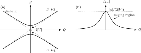
An avoided crossing separates the adiabatic energies $E_\pm(Q)$ by $2\lvert V\rvert$. The derivative coupling $\lvert d_{+-}(Q)\rvert$ peaks in the same narrow region, so a nuclear packet can change electronic character even though its coordinate motion is slow.

This model isolates the local mechanism behind Landau–Zener transitions, but the two descriptions answer different questions. The Born–Oppenheimer channel equations describe how nuclear kinetic energy couples coordinate-dependent electronic states. A Landau–Zener formula additionally assumes a prescribed passage, usually with a locally linear time dependence, and estimates a transition probability. It should not replace a check of the molecular wavepacket, the dimensionality of the crossing region, or the validity of the two-state truncation.

Where the Approximation Fails

Single-surface dynamics becomes suspect in several recurring situations:

• Avoided crossings: a small gap produces sharply varying electronic eigenvectors and enhanced derivative couplings.
• Conical intersections: two surfaces become degenerate in a multidimensional nuclear space, so one isolated electronic line bundle no longer describes the crossing region.
• Fast or energetic nuclei: collisions, photodissociation, and highly excited vibrations can increase the momentum-dependent coupling.
• Light nuclei: hydrogen transfer and proton-coupled electron transfer can make nuclear delocalization and nonadiabatic effects especially important.
• Broad wavepackets: a packet centered in a benign region may still overlap a small-gap region through its tails.
• Ionization or dense electronic spectra: separation from electronic continua or nearby Rydberg manifolds can fail.
• Strong time-dependent driving: the relevant quasienergy or dressed-state gaps can differ from field-free electronic gaps.

An exact degeneracy does not automatically imply a transition between every pair of states. Symmetry may block the matrix element, and a degenerate multiplet can sometimes be retained as a whole while remaining isolated from all other states. In that case the correct effective theory is matrix valued rather than a scalar one-surface theory.

Berry Phase Preview

For an isolated electronic state, the diagonal derivative coupling defines a local Berry connection

$$\mathbf A_a(R) = i\langle\phi_a(R)\vert \nabla_R\phi_a(R)\rangle_e.$$

If the nuclei traverse a closed loop $C$, the electronic state can acquire the holonomy

$$\gamma_a(C)=\oint_C\mathbf A_a(R)\mathbin{\cdot}dR.$$

Locally one can often choose a phase convention with $\mathbf A_a=0$, especially for a real nondegenerate electronic Hamiltonian. Globally, a loop around a conical intersection may obstruct one single-valued choice and produce a nontrivial phase. That phase changes nuclear boundary conditions and interference even when the trajectory remains on one adiabatic surface.

The canonical derivation of the covariant nuclear momentum, gauge transformations, Born–Huang scalar term, and conical-intersection holonomy is on Born–Oppenheimer Berry Phase. The present page needs only the methodological warning: “neglect transitions” does not imply “neglect geometry.”

Relation to Other Slow–Fast Methods

Born–Oppenheimer theory belongs to the same family as projection methods, adiabatic following, and dynamical elimination, but its retained variables and expansion are distinctive.

Method	Slow object	Fast structure	Characteristic output
Born–Oppenheimer	Nuclear wavefunction	Coordinate-dependent electronic eigenspace	Potential surfaces and derivative couplings
Adiabatic approximation	Amplitude in an instantaneous eigenspace	Slowly varying Hamiltonian in time	Eigenstate following and transition estimates
Adiabatic elimination	Slow amplitudes or density operator	Fast detuned or rapidly relaxing sector	Local effective generator and induced couplings
Projection methods	Chosen model subspace	Complementary Hilbert subspace	Energy-dependent self-energy and reconstruction

Treating a nuclear trajectory $R(t)$ as prescribed converts electronic following into a time-dependent adiabatic problem, with

$$\frac{d}{dt}\lvert\phi_a(R(t))\rangle = \sum_A\dot R_A\mathbin{\cdot} \nabla_A\lvert\phi_a(R)\rangle.$$

That is useful for intuition and mixed quantum–classical schemes. The full Born–Oppenheimer problem is richer because $R$ is itself an operator and a quantum coordinate. Nuclear branching, tunneling, interference, and geometric phase cannot in general be represented by one prescribed path.

A Practical Validity Workflow

1. Define the internal Hamiltonian. Remove center-of-mass motion as appropriate and state whether internuclear repulsion is included in $H_e(R)$.
2. Specify the target states and observable. Bound levels, short-time wavepacket motion, a scattering amplitude, and a reaction probability can require different controls.
3. Identify an electronic state or cluster. Map the gaps to excluded channels over the entire nuclear region that can be reached.
4. Inspect derivative couplings or projectors. A visually large surface gap is not enough if the eigenvectors vary rapidly; a small gap can be harmless only when coupling is forbidden or the full cluster is retained.
5. Estimate nuclear phase-space support. Use momenta and spatial tails, not only the mean geometry and mean velocity.
6. Compare first- and second-derivative couplings with gaps. Diagnostics such as $\eta_{ab}$ and $\zeta_{ab}$ reveal likely failure regions.
7. Choose the effective description. Use one surface, one surface with diagonal/geometric corrections, or a coupled multisurface model.
8. Test stability. Enlarge the electronic channel set, vary the nuclear energy window, and check whether the observable is stable on the required time scale.

This workflow turns a qualitative timescale story into a falsifiable approximation.

Common Mistakes

• Saying the approximation “fixes the nuclei.” Only the auxiliary electronic eigenproblem holds $R$ fixed; the nuclear equation remains quantum mechanical.
• Treating the product $\chi(R)\phi(r;R)$ as exact while forgetting that $T_N$ differentiates both factors.
• Quoting only the electron-to-nuclear mass ratio and never checking electronic gaps or derivative couplings.
• Assuming every potential-energy surface is globally smooth and nondegenerate.
• Dropping diagonal geometric terms merely because off-diagonal transitions are small.
• Comparing the gap only at the equilibrium geometry when the nuclear wavefunction explores a wider region.
• Using Hellmann–Feynman forces from an incomplete variational or geometry-dependent basis without the required response terms.
• Calling a multisurface calculation “beyond Born–Oppenheimer” without stating which derivative couplings and nuclear quantum effects are retained.
• Confusing the Born–Oppenheimer approximation with a classical-nuclei molecular-dynamics approximation.

References

• M. Born and R. Oppenheimer, “Zur Quantentheorie der Molekeln,” Annalen der Physik 389, 457–484 (1927), doi:10.1002/andp.19273892002.
• M. Born and K. Huang, Dynamical Theory of Crystal Lattices, Clarendon Press (1954).
• G. A. Hagedorn, “A time dependent Born–Oppenheimer approximation,” Communications in Mathematical Physics 77, 1–19 (1980).
• C. A. Mead and D. G. Truhlar, “On the determination of Born–Oppenheimer nuclear motion wave functions including complications due to conical intersections and identical nuclei,” The Journal of Chemical Physics 70, 2284–2296 (1979), doi:10.1063/1.437734.
• H. Spohn and S. Teufel, “Adiabatic decoupling and time-dependent Born–Oppenheimer theory,” Communications in Mathematical Physics 224, 113–132 (2001).
• G. Panati, H. Spohn, and S. Teufel, “The time-dependent Born–Oppenheimer approximation,” ESAIM: Mathematical Modelling and Numerical Analysis 41, 297–314 (2007), doi:10.1051/m2an:2007023.
• D. R. Yarkony, “Diabolical conical intersections,” Reviews of Modern Physics 68, 985–1013 (1996), doi:10.1103/RevModPhys.68.985.
• B. T. Sutcliffe and R. G. Woolley, “On the quantum theory of molecules,” The Journal of Chemical Physics 137, 22A544 (2012), doi:10.1063/1.4755287.
• T. Jecko, “On the mathematical treatment of the Born–Oppenheimer approximation,” Journal of Mathematical Physics 55, 053504 (2014), doi:10.1063/1.4870855.

Exercises

1. Derive the coupled-channel equations

Starting from

$$\Psi(r,R)=\sum_b\chi_b(R)\phi_b(r;R),$$

apply $T_N$ and project onto $\langle\phi_a(R)\rvert$. Derive all three nuclear derivative terms and explain which ones survive if the electronic basis is independent of $R$.

Solution

For each nucleus,

$$\begin{aligned} \nabla_A^2(\chi_b\phi_b) ={}& \phi_b\nabla_A^2\chi_b \\ &+ 2(\nabla_A\phi_b)\mathbin{\cdot}\nabla_A\chi_b \\ &+ \chi_b\nabla_A^2\phi_b. \end{aligned}$$

Multiplying by $-\hbar^2/(2M_A)$, summing over $A$ and $b$, and taking the electronic inner product with $\phi_a$ gives

$$\begin{aligned} \sum_b\mathcal H_{ab}^{N}\chi_b &= E\chi_a, \\ \mathcal H_{ab}^{N} &= -\sum_A\frac{\hbar^2}{2M_A}\mathcal K_{ab}^{A} \\ &\quad+ E_a\delta_{ab}, \\ \mathcal K_{ab}^{A} &= \delta_{ab}\nabla_A^2 +2\mathbf d_{ab}^{A}\mathbin{\cdot}\nabla_A +\tau_{ab}^{A}. \end{aligned}$$

If the basis is independent of $R$, then $\mathbf d_{ab}^{A}=\tau_{ab}^{A}=0$. Only the ordinary nuclear kinetic term remains. In the molecular electronic eigenbasis, however, $R$ dependence is precisely what converts electronic energies into surfaces, so the derivative terms are generally present.

2. Gap dependence of derivative coupling

Differentiate

$$H_e(R)\lvert\phi_b(R)\rangle = E_b(R)\lvert\phi_b(R)\rangle$$

with respect to $R_A$. Project onto $\langle\phi_a\rvert$ for $a\ne b$ and derive the off-diagonal Hellmann–Feynman identity.

Solution

Differentiation gives

$$\begin{aligned} (\nabla_AH_e)\lvert\phi_b\rangle &+ H_e\lvert\nabla_A\phi_b\rangle \\ &= (\nabla_AE_b)\lvert\phi_b\rangle \\ &\quad+ E_b\lvert\nabla_A\phi_b\rangle. \end{aligned}$$

Projecting with $\langle\phi_a\rvert$, using orthogonality and $\langle\phi_a\rvert H_e=E_a\langle\phi_a\rvert$, yields

$$\langle\phi_a\vert\nabla_AH_e\vert\phi_b\rangle +E_a\mathbf d_{ab}^{A} = E_b\mathbf d_{ab}^{A}.$$

Therefore

$$\mathbf d_{ab}^{A} = \frac{ \langle\phi_a\vert\nabla_AH_e\vert\phi_b\rangle }{ E_b-E_a }.$$

The identity assumes distinct differentiable eigenvalues at the point in question. At a degeneracy, one should work with the degenerate projector or a retained multiplet.

3. Two-state avoided crossing

For

$$H_e(Q)=\alpha Q\,\sigma_z+V\sigma_x,$$

find the eigenvalues and show that

$$\left\lvert d_{+-}(Q)\right\rvert = \frac{\lvert\alpha V\rvert}{ 2(\alpha^2Q^2+V^2) }.$$

Where is the one-surface approximation most vulnerable?

Solution

The characteristic equation is

$$E^2=\alpha^2Q^2+V^2,$$

so $E_\pm=\pm\sqrt{\alpha^2Q^2+V^2}$. Introduce a mixing angle $\theta(Q)$ through

$$\tan 2\theta(Q)=\frac{V}{\alpha Q}.$$

For a consistent real choice of eigenvectors, the off-diagonal derivative coupling has magnitude $\lvert\theta'(Q)\rvert$. Differentiating gives

$$\left\lvert\theta'(Q)\right\rvert = \frac{\lvert\alpha V\rvert}{ 2(\alpha^2Q^2+V^2) }.$$

It peaks at $Q=0$, where the adiabatic gap is smallest. The combined diagnostic $\eta_{+-}$ is also maximal there and scales as $V^{-2}$ at fixed velocity and slope. The narrow-gap region is therefore the most vulnerable.

4. Why the fourth root appears

In atomic units, consider one nuclear normal coordinate near a minimum:

$$H_N = -\frac{\mu}{2}\frac{d^2}{dQ^2} +\frac{KQ^2}{2},$$

where $K$ is of order unity and $\mu=m_e/M$. Determine the scaling of the oscillator frequency, ground-state width, and zero-point energy with $\mu$. Express the result using $\kappa=\mu^{1/4}$.

Solution

The effective mass is $1/\mu$, so

$$\omega=\sqrt{\mu K}\sim\mu^{1/2}.$$

The ground-state width scales as

$$\Delta Q \sim \sqrt{\frac{1}{(1/\mu)\omega}} \sim \mu^{1/4},$$

up to factors involving $K$. The zero-point energy scales as

$$E_0=\frac{\omega}{2}\sim\mu^{1/2}.$$

With $\kappa=\mu^{1/4}$, the displacement is of order $\kappa$ and the vibrational energy is of order $\kappa^2$. This is why the original molecular expansion naturally uses a fourth-root parameter even though the nuclear kinetic prefactor is $\mu=\kappa^4$.

5. Gauge change in one electronic channel

Let

$$\lvert\phi_a(R)\rangle \longrightarrow e^{i\vartheta(R)} \lvert\phi_a(R)\rangle.$$

How must $\chi_a(R)$ transform so that the molecular product is unchanged? Find the transformation of $\mathbf A_a=i\langle\phi_a\vert\nabla_R\phi_a\rangle_e$.

Solution

The product $\chi_a\phi_a$ is invariant if

$$\chi_a(R)\longrightarrow e^{-i\vartheta(R)}\chi_a(R).$$

The transformed connection is

$$\begin{aligned} \mathbf A_a' &= i\langle\phi_a\vert e^{-i\vartheta} \nabla_R\!\left(e^{i\vartheta}\phi_a\right) \rangle_e \\ &= \mathbf A_a-\nabla_R\vartheta. \end{aligned}$$

Consequently, only gauge-covariant combinations in the nuclear Hamiltonian and closed-loop holonomies are physical. A local gauge with $\mathbf A_a=0$ need not extend globally around a degeneracy.

6. Diagnose the approximation

A nuclear wavepacket starts near a stable minimum on the electronic ground surface. Its mean geometry is far from an avoided crossing, but a photoexcitation gives it enough kinetic energy that part of the packet reaches the crossing region. List the checks needed before using one ground-state surface for the subsequent dynamics.

Solution

One should check:

1. the minimum electronic gap over the full spatial support reached by the packet, including its tails;
2. the first- and second-derivative couplings in the crossing region;
3. the momentum distribution there, since the leading coupling is proportional to nuclear velocity;
4. whether a two-surface or larger electronic cluster remains isolated from all other states;
5. whether the observable and propagation time are sensitive to a small transferred amplitude;
6. whether geometric phase or interference matters for paths around the crossing;
7. stability of the result when the coupled-channel basis is enlarged.

The benign mean geometry is not enough. If appreciable support reaches the narrow-gap region with substantial momentum, a coupled-surface treatment is the natural starting point.