Effective Hamiltonians in Quantum Matter

Quantum matter is full of Hamiltonians that are not microscopic starting points. A spin model can emerge from itinerant electrons whose charge motion is energetically suppressed. A narrow band can behave like a particle with a mass different from the bare electron mass. A projected band can acquire longer-range hopping, exchange, and geometric terms that were not obvious in the original basis.

An effective Hamiltonian in quantum matter acts on the degrees of freedom that remain active below a chosen energy, momentum, or length scale. The eliminated states still matter through virtual processes, renormalized parameters, induced interactions, and dressed observables.

This page is a bridge to many-body and condensed-matter applications. It owns the exact Hubbard-dimer superexchange benchmark and the band effective-mass application. Effective Hamiltonians in Many-Body Systems owns the lattice-scale Hubbard-to-Heisenberg and Anderson-to-Kondo reductions, generated operators, locality, and many-body validity audit. Hubbard Model owns the parent model definition, Heisenberg Model owns the resulting spin model and its conventions, and Effective Mass owns the band-curvature formula.

Low-Energy Subspaces in Many-Body Systems

Write

$$H = H_0+V,$$

and let $P$ project onto a low-energy eigenspace of $H_0$ with energy $E_0$. The complementary projector

$$Q=I-P$$

contains high-energy charge configurations, upper orbitals, remote bands, ligand excitations, or other degrees of freedom that will be eliminated.

If

$$Q(H_0-E_0)Q \ge \Delta Q$$

with $\Delta\gt0$, then the leading energy-independent effective Hamiltonian is

$$H_{\mathrm{eff}} = E_0P + PVP + H_{\mathrm{eff}}^{(2)} + O\!\left( \frac{V^3}{\Delta^2} \right),$$

where

$$H_{\mathrm{eff}}^{(2)} = - PVQ R_Q QVP$$

and

$$R_Q = \left[ Q(H_0-E_0)Q \right]^{-1}.$$

The inverse is taken only on $Q\mathcal H$. The minus sign says that coupling to higher-energy states lowers an isolated retained level at second order. When the retained manifold has a nonzero bandwidth or several unperturbed energies, one uses the corresponding resolvent or a symmetrized Schrieffer–Wolff expression.

Many-body projection differs from a one-state perturbation problem in three important ways:

1. The retained space can be exponentially large and highly degenerate.
2. The perturbation can connect many local configurations even when each local matrix element is small.
3. Projection generates new many-site operators rather than only shifting a few energy levels.

The useful small parameter is therefore usually local, such as

$$\eta_{\mathrm{loc}} \sim \frac{\lvert t\rvert}{U},$$

not the ratio of global operator norms, which often grows with system size. A controlled expansion must still account for coordination number, bandwidth, resonances, and the order at which the desired process first appears.

The low-energy sector need not itself be gapped. A gap of order $U$ can separate charge excitations in $Q$ while spin excitations inside $P$ remain gapless in the thermodynamic limit. The projection controls separation between sectors, not the infrared physics within the retained sector.

Superexchange on a Hubbard Dimer

The two-site Hubbard model is the smallest exact benchmark for interaction-generated spin exchange. With two sites and spin-conserving hopping,

$$H = H_U+T,$$

where

$$H_U = U \sum_{i=1}^{2} n_{i\uparrow}n_{i\downarrow}$$

and

$$T = - t \sum_{\sigma} \left( c_{1\sigma}^\dagger c_{2\sigma} + c_{2\sigma}^\dagger c_{1\sigma} \right).$$

Assume repulsive interaction $U\gt0$ and exactly two electrons. The low-energy sector $P$ contains one electron on each site. It has one spin singlet and three spin triplets. The eliminated sector $Q$ contains a doubly occupied site and an empty site, at unperturbed energy $U$.

Hopping changes the number of doubly occupied sites, so

$$PTP=0.$$

A singlet can hop virtually into a doublon–hole configuration and return. A triplet cannot place two electrons in the same spatial orbital because the required onsite spin state would violate fermionic antisymmetry.

After choosing the phase of the doublon combination that couples to the singlet, the nontrivial singlet block is

$$H_{\mathrm{singlet}} = \begin{pmatrix} 0 & -2t\\ -2t & U \end{pmatrix}.$$

Its exact eigenvalues are

$$E_{\pm} = \frac{1}{2} \left( U \pm \sqrt{U^2+16t^2} \right).$$

The low-energy singlet therefore has

$$\begin{aligned} E_S &= \frac{1}{2} \left( U-\sqrt{U^2+16t^2} \right) \\ &= - \frac{4t^2}{U} + \frac{16t^4}{U^3} + O\!\left( \frac{t^6}{U^5} \right). \end{aligned}$$

The triplets remain at zero energy in this convention. The singlet–triplet splitting is

$$J_{\mathrm{exact}} = \frac{ \sqrt{U^2+16t^2}-U }{2},$$

whose leading strong-coupling limit is

$$J = \frac{4t^2}{U}.$$

Because $J\gt0$, the simple repulsive one-band Hubbard dimer produces antiferromagnetic exchange.

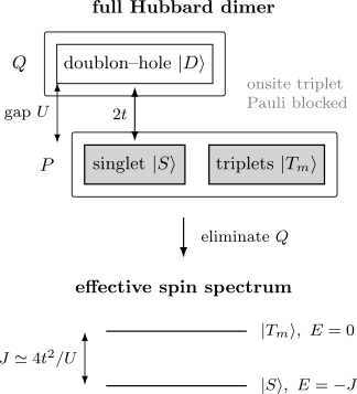
At half filling, the retained sector $P$ has one electron per site. Only the spin singlet couples to the doublon–hole sector $Q$ through spin-conserving hopping. Eliminating the energy cost $U$ lowers the singlet by $J=4t^2/U+O(t^4/U^3)$ and leaves the triplets higher.

For example, at

$$U=8\lvert t\rvert,$$

second order gives $J=0.5\lvert t\rvert$, while the exact splitting is approximately

$$J_{\mathrm{exact}} \simeq 0.472\lvert t\rvert.$$

The comparison is a useful reminder that identifying the right effective operator does not guarantee that its lowest-order coefficient is numerically precise.

From the Dimer Benchmark to Lattice Models

The exact dimer calculation above fixes the sign and leading scale of one virtual bond process:

$$J = \frac{4|t|^2}{U} >0.$$

For dimensionless spin operators, the corresponding bond term is

$$H_{ij}^{(2)} = J \left( \mathbf s_i\cdot\mathbf s_j - \frac14 \right).$$

Extending that result to a lattice requires more than copying the coefficient. One must define the no-doublon projector, decide whether projected hopping survives, sum every virtual path, retain same-order density and correlated-hopping terms, and control locality as the system grows.

Effective Hamiltonians in Many-Body Systems is the canonical derivation of that lattice reduction. It explains why:

• a half-filled no-doublon sector has $PTP=0$ and reduces to antiferromagnetic spin exchange at second order;
• a doped no-doublon sector has $PTP\ne0$ and retains projected hopping at first order;
• the bond density term is constant only at fixed half filling;
• three-site terms arise at the same order as exchange in the doped expansion;
• higher orders and additional microscopic structure generate longer-range, ring, anisotropic, or flux-sensitive interactions.

The Heisenberg Model owns the resulting spin problem. The t–J Model Preview owns constrained hopping and the doped effective model. This page retains the dimer as an exact finite-system benchmark for the coefficient and truncation error.

Effective Mass as Band-Space Reduction

Scale separation also occurs in momentum space. Let a periodic one-particle Hamiltonian have Bloch energies

$$E_n(\mathbf k).$$

Suppose band $n$ is isolated from other bands near $\mathbf k_0$ and has an extremum there. Write

$$\mathbf q = \mathbf k-\mathbf k_0.$$

The local band expansion is

$$\begin{aligned} E_n(\mathbf k_0+\mathbf q) \simeq{}& E_n(\mathbf k_0) \\ &+ \frac{\hbar^2}{2} \sum_{i,j} (m^{-1})_{ij} q_iq_j, \end{aligned}$$

where

$$(m^{-1})_{ij} = \frac{1}{\hbar^2} \frac{\partial^2E_n}{ \partial k_i\,\partial k_j } \biggr\rvert_{\mathbf k_0}.$$

For a slowly varying external potential $V_{\mathrm{slow}}(\mathbf r)$ and constant mass tensor, the envelope function obeys the effective Hamiltonian

$$H_{\mathrm{env}} = E_n(\mathbf k_0) + V_{\mathrm{slow}}(\mathbf r) + T_{\mathrm{eff}},$$

where

$$T_{\mathrm{eff}} = \frac{1}{2} \sum_{i,j} p_i (m^{-1})_{ij} p_j, \qquad p_i=-i\hbar\partial_i.$$

The rapidly varying lattice-scale Bloch structure has been encoded into the band edge, effective mass, and envelope basis. The result resembles a free-particle Hamiltonian, but $m^\ast$ is a property of a chosen band, direction, and expansion point.

For a one-dimensional nearest-neighbor tight-binding band

$$E(k) = \epsilon_0 - 2t_{\mathrm h}\cos(ka),$$

with $t_{\mathrm h}\gt0$, expansion near $k=0$ gives

$$E(k) \simeq \epsilon_0-2t_{\mathrm h} + t_{\mathrm h}a^2k^2.$$

Matching the quadratic term to $\hbar^2k^2/(2m^\ast)$ yields

$$m^\ast = \frac{\hbar^2}{ 2t_{\mathrm h}a^2 }.$$

Near the band maximum at $k=\pi/a$, the electron curvature and effective mass are negative. Hole variables reorganize that physics into positive-energy carriers with their own charge and mass conventions.

Validity of a single-band mass

The scalar or tensor effective-mass Hamiltonian requires:

1. a smooth isolated band or isolated group of bands;
2. wave packets localized in momentum near the expansion point;
3. external potentials varying slowly on the lattice scale;
4. energies small enough that nonparabolic terms are negligible;
5. no unresolved degeneracy requiring a multiband Hamiltonian.

Near band crossings, strong spin–orbit mixing, or topologically nontrivial degeneracies, a multiband $k\cdot p$ Hamiltonian and Berry-connection terms may be essential. Interactions can also renormalize quasiparticle dispersion, producing a many-body effective mass distinct from the bare band-curvature mass.

Bloch Theorem owns the translation-symmetry statement, while Effective Mass owns the formula and its common response-dependent variants.

Projection Changes Operators

An effective Hamiltonian does not make the physical state literally remain in the bare retained sector. If a Schrieffer–Wolff transformation $e^S$ block diagonalizes the Hamiltonian, an observable must be transformed as

$$O_{\mathrm{eff}} = P e^S O e^{-S}P.$$

For the large-$U$ Hubbard model, the bare double-occupancy operator

$$D = \sum_i n_{i\uparrow}n_{i\downarrow}$$

satisfies

$$PDP=0.$$

Nevertheless, a physical low-energy eigenstate contains virtual doublon–hole weight of order $(t/U)^2$, so its double occupancy is small rather than exactly zero. Projecting the state while leaving the observable bare would miss that contribution.

The same rule applies to current operators, spin operators, polarization, density, and optical matrix elements. Effective spectra can be correct while effective response functions are wrong if the probes are not dressed consistently.

Symmetry, Locality, and Nonuniqueness

Three structural checks are especially useful in quantum matter:

Symmetry. If $H$, $P$, and the block-diagonalization procedure respect a symmetry, $H_{\mathrm{eff}}$ should inherit it. An unexpected symmetry-breaking term may signal an algebra error or a projector that was not symmetry invariant.

Locality. Eliminating local high-energy processes generally produces quasi-local interactions of increasing range and body order. Truncating those terms requires an order and range estimate. A short effective Hamiltonian is not automatically the most accurate one.

Internal unitary freedom. Two effective Hamiltonians can differ by a unitary transformation acting entirely within $P$. Their coefficients may look different while spectra and consistently transformed observables agree. Comparisons between derivations must first align basis and gauge conventions.

These points become more important with system size. A local expansion in $t/U$ may be meaningful even though the norm of the total hopping Hamiltonian is extensive. Rigorous many-body control then uses locality, linked processes, or quasi-local transformations rather than a volume-independent bound on the full operator norm.

Practical Workflow

For a low-energy quantum-matter reduction:

1. Specify the microscopic or parent Hamiltonian and its conventions.
2. Define $P$ by filling, band, charge sector, orbital manifold, or energy window.
3. Identify the gap or penalty separating $P$ from $Q$.
4. Determine whether $PVP$ vanishes or contains first-order dynamics.
5. Derive every operator through the desired order, including constants and density terms.
6. Preserve symmetries and track newly generated interactions.
7. Transform observables and states, not only the Hamiltonian.
8. Benchmark spectra and matrix elements against a dimer, cluster, or larger-band calculation.
9. Test the expansion over the full parameter, momentum, temperature, and drive range of interest.
10. Enlarge the retained space when a denominator becomes small.

At present, Math Needed for Many-Body Quantum Mechanics and Math Needed for Quantum Matter provide the routes into existing prerequisites. The future volumes will own lattice-model solution methods, phases of matter, material exchange mechanisms, quasiparticles, transport, and band topology.

Common Mistakes

• Replacing $H$ by $PHP$ and missing virtual exchange.
• Treating $t/U$ as the only scale while ignoring bandwidth, coordination, filling, temperature, and drive frequency.
• Calling every antiferromagnetic coupling $4t^2/U$ without specifying the one-band Hubbard assumptions.
• Dropping the $-n_in_j/4$ term before fixing the filling.
• Using a Heisenberg model away from half filling while discarding allowed projected hopping.
• Omitting three-site terms without naming the additional t–J model approximation.
• Setting double occupancy exactly to zero for physical dressed states.
• Confusing band effective mass with bare electron mass or interaction-renormalized quasiparticle mass.
• Applying a one-band mass tensor at a degeneracy or far from the expansion point.
• Comparing effective Hamiltonian coefficients without aligning low-energy basis conventions.

Cross-Links

• Effective Hamiltonians and Scale Separation
• Projection Methods
• Schrieffer–Wolff Transformation
• High-Frequency Expansions
• Hubbard Model
• Hubbard Physics in Materials
• Effective Hamiltonians in Many-Body Systems
• Hubbard Model Glossary Entry
• Hubbard Model Hamiltonian
• Heisenberg Model
• t–J Model Preview
• Heisenberg Chain Model Card
• Tight-Binding Dimer
• Many-Particle Hamiltonians
• Fermionic Anticommutation Relations
• Bloch Theorem
• Effective Mass
• Math Needed for Many-Body Quantum Mechanics
• Math Needed for Quantum Matter

References

1. J. Hubbard, “Electron correlations in narrow energy bands,” Proceedings of the Royal Society A 276, 238–257 (1963).
2. P. W. Anderson, “Antiferromagnetism. Theory of superexchange interaction,” Physical Review 79, 350–356 (1950).
3. P. W. Anderson, “New approach to the theory of superexchange interactions,” Physical Review 115, 2–13 (1959).
4. M. Takahashi, “Half-filled Hubbard model at low temperature,” Journal of Physics C: Solid State Physics 10, 1289–1301 (1977).
5. A. H. MacDonald, S. M. Girvin, and D. Yoshioka, “$t/U$ expansion for the Hubbard model,” Physical Review B 37, 9753–9756 (1988).
6. S. Bravyi, D. P. DiVincenzo, and D. Loss, “Schrieffer–Wolff transformation for quantum many-body systems,” Annals of Physics 326, 2793–2826 (2011).
7. J. M. Luttinger and W. Kohn, “Motion of electrons and holes in perturbed periodic fields,” Physical Review 97, 869–883 (1955).
8. A. Auerbach, Interacting Electrons and Quantum Magnetism, Springer (1994).

Exercises

Exact dimer expansion

Expand the exact Hubbard-dimer singlet–triplet splitting

$$J_{\mathrm{exact}} = \frac{ \sqrt{U^2+16t^2}-U }{2}$$

through order $t^4/U^3$. Does second order overestimate or underestimate the exact splitting for finite $t/U$?

Solution

For $U\gt0$,

$$\sqrt{U^2+16t^2} = U \sqrt{ 1+\frac{16t^2}{U^2} }.$$

Using

$$\sqrt{1+x} = 1+\frac{x}{2}-\frac{x^2}{8}+O(x^3),$$

gives

$$\begin{aligned} \sqrt{U^2+16t^2} ={}& U + \frac{8t^2}{U} \\ &- \frac{32t^4}{U^3} + O\!\left( \frac{t^6}{U^5} \right). \end{aligned}$$

Therefore

$$J_{\mathrm{exact}} = \frac{4t^2}{U} - \frac{16t^4}{U^3} + O\!\left( \frac{t^6}{U^5} \right).$$

The first correction is negative, so the second-order value $4t^2/U$ overestimates the exact splitting at finite $t/U$.

Singlet projector

For two dimensionless spin-$1/2$ operators, prove that

$$P_S = \frac{1}{4} - \mathbf s_1\cdot\mathbf s_2$$

is the projector onto the singlet.

Solution

Use

$$\mathbf s_{\mathrm{tot}}^2 = \mathbf s_1^2 + \mathbf s_2^2 + 2\mathbf s_1\cdot\mathbf s_2.$$

For spin $1/2$,

$$\mathbf s_1^2 = \mathbf s_2^2 = \frac{3}{4}.$$

The singlet has total spin zero, so

$$\mathbf s_1\cdot\mathbf s_2 = - \frac{3}{4}.$$

The triplet has total spin one and $\mathbf s_{\mathrm{tot}}^2=2$, so

$$\mathbf s_1\cdot\mathbf s_2 = \frac{1}{4}.$$

Thus $1/4-\mathbf s_1\cdot\mathbf s_2$ has eigenvalue $1$ on the singlet and $0$ on every triplet. It is therefore the singlet projector.

Exchange convention

Rewrite

$$J\mathbf s_i\cdot\mathbf s_j$$

using physical spin operators $\mathbf S_i=\hbar\mathbf s_i$. What units must the coefficient multiplying $\mathbf S_i\cdot\mathbf S_j$ have?

Solution

Substitution gives

$$J\mathbf s_i\cdot\mathbf s_j = \frac{J}{\hbar^2} \mathbf S_i\cdot\mathbf S_j.$$

Since $\mathbf S_i\cdot\mathbf S_j$ has units of $\hbar^2$, its coefficient must have units of energy divided by $\hbar^2$. The symbol called “exchange coupling” therefore has different dimensions in the dimensionless-spin and physical-spin conventions.

Why doping restores first-order hopping

Explain why $PTP=0$ at half filling in the no-double-occupancy sector but need not vanish when a hole is present.

Solution

At half filling with one electron per site, every nearest-neighbor hop places an electron on an already occupied site. The resulting state has one doublon and one hole, so it lies in $Q$ and is removed by the final projector $P$.

If a hole is present, an electron can hop from an occupied site into the empty site without creating double occupancy. Both the initial and final states remain in $P$, so the matrix element survives in $PTP$. This projected hopping appears at order $t$, while exchange still appears at order $t^2/U$.

Tight-binding effective mass

For

$$E(k) = \epsilon_0 - 2t_{\mathrm h}\cos(ka),$$

compute the effective mass at $k=0$ and $k=\pi/a$.

Solution

The curvature is

$$\frac{d^2E}{dk^2} = 2t_{\mathrm h}a^2\cos(ka).$$

Therefore

$$m^\ast(0) = \frac{\hbar^2}{ 2t_{\mathrm h}a^2 },$$

while

$$m^\ast(\pi/a) = - \frac{\hbar^2}{ 2t_{\mathrm h}a^2 }.$$

The negative electron mass at the band maximum signals that a hole description may be more convenient there.

Virtual double occupancy

Why can a physical low-energy Hubbard eigenstate have double occupancy of order $(t/U)^2$ even though $PDP=0$ in the projected spin space?

Solution

The block-diagonal low-energy state is related to the physical state by the inverse Schrieffer–Wolff transformation. Its $Q$-sector amplitude is first order in $t/U$ because one hop creates a virtual doublon–hole pair. Probability is amplitude squared, so the physical double occupancy scales as

$$\left( \frac{t}{U} \right)^2.$$

Equivalently, transforming the observable produces

$$D_{\mathrm{eff}} = P e^S D e^{-S}P,$$

whose leading nonzero term is second order even though $PDP=0$.