Addition of Angular Momentum

Angular momentum addition is the representation-theoretic organization of a composite Hilbert space under joint rotations. Two subsystems first form a tensor product. The generator of the same physical rotation acting on both factors is the sum of their angular momenta, and the tensor-product representation decomposes into irreducible sectors labeled by total $J$.

The word addition therefore refers to several related operations that should not be collapsed into one:

• tensoring the subsystem Hilbert spaces;
• adding the generators component by component;
• decomposing the resulting rotation representation into total-$J$ sectors;
• changing between uncoupled and coupled bases;
• choosing a coupling order when three or more angular momenta are present.

This chapter develops those operations as a coherent workflow. It begins with the symmetry action, uses two spin-$1/2$ systems as the first complete example, and then moves to orbital-plus-spin coupling, spectroscopy-oriented coupling schemes, Wigner symbols, and the exchange-symmetry preview.

Canonical Boundaries

This page owns the chapter map and the structural relation among the results. The detailed derivations and application-specific physics remain at their canonical homes.

Topic	Canonical home	Role here
tensor-product rotation action	Tensor Product Representations	identifies the composite representation and its irreducible decomposition
total generator	Total Angular Momentum	owns the operator sum and conservation laws
basis dictionary	Coupled and Uncoupled Bases	compares the two complete commuting sets
first explicit decomposition	Two Spin-1/2 Particles	constructs the four coupled states
rotational meaning of scalar and vector sectors	Singlet and Triplet States	owns projectors, correlations, and joint rotations
numerical basis transformation	Clebsch–Gordan Coefficients	defines and computes the coefficients
convention-safe lookup	Clebsch–Gordan Tables and Conventions	fixes phases, ordering, and table workflow
physically adapted coupling orders	Angular Momentum Coupling Schemes	compares LS, jj, hyperfine, and molecular schemes
scalar orbital-spin interaction	Spin–Orbit Coupling	diagonalizes $\mathbf L\cdot\mathbf S$ with total $J$
one-particle orbital-spin basis	Addition of Orbital and Spin Angular Momentum	owns $\ell\otimes s$ labels and spinor spherical harmonics
changes of coupling order	Recoupling and Wigner Symbols	introduces $3j$, $6j$, and $9j$ symbols
identical-particle consequence	Identical Particles and Exchange Symmetry Preview	connects spin-sector symmetry to the later full treatment

The general tensor-product formalism belongs to Tensor Products. Entanglement, Bell states, and the symmetrization postulate belong to Composite Systems. Large coefficient tables belong to the Reference, while this chapter explains what the numbers mean and how to use them consistently.

Composite Rotations Start with a Tensor Product

If two subsystems carry irreducible angular momenta $j_1$ and $j_2$, their joint Hilbert space is

$$\mathcal H = \mathcal H_{j_1} \otimes \mathcal H_{j_2}.$$

Its dimension is

$$\dim\mathcal H = (2j_1+1)(2j_2+1).$$

A single physical rotation $R$ of the composite system acts diagonally:

$$U(R) = U_1(R)\otimes U_2(R).$$

The same $R$ appears on both factors. This is not an arbitrary pair of independent local unitaries. Angular momentum addition classifies the state space under this joint rotational action.

The tensor product remains the composite space even after it is decomposed into total-$J$ sectors. Product states, entangled states, and coupled eigenstates are all vectors in this same Hilbert space.

Total Angular Momentum Is the Joint Generator

Differentiating the joint rotation gives

$$J_i = J_{1i}\otimes I_2 + I_1\otimes J_{2i}.$$

In compact notation,

$$\mathbf J=\mathbf J_1+\mathbf J_2.$$

The identity factors are implicit but essential: each subsystem operator acts nontrivially only on its own factor. Operators on different factors commute,

$$\left[ J_{1i}\otimes I_2, I_1\otimes J_{2j} \right] = 0,$$

so the total components satisfy

$$[J_i,J_j] = i\hbar \sum_k\epsilon_{ijk}J_k.$$

The total operator is therefore an angular momentum in its own right. It generates simultaneous rotations and admits the usual Casimir $J^2$ and projection $J_z$.

Two identities drive most calculations:

$$J_z=J_{1z}+J_{2z},$$

and

$$J^2 = J_1^2+J_2^2 + 2\mathbf J_1\cdot\mathbf J_2.$$

The first makes magnetic projections additive. The second explains why a product state with definite $m_1,m_2$ is usually not an eigenstate of total $J^2$.

Irreducible Decomposition and the Triangle Rule

For two $SU(2)$ angular momenta, the tensor product decomposes as

$$\mathcal H_{j_1}\otimes\mathcal H_{j_2} \cong \bigoplus_{J=|j_1-j_2|}^{j_1+j_2} \mathcal H_J.$$

Equivalently, the allowed total angular momenta are

$$\begin{gathered} J=|j_1-j_2|, \\ |j_1-j_2|+1, \ldots, j_1+j_2. \end{gathered}$$

Each allowed $J$ occurs once when exactly two irreducible angular momenta are coupled. For each $J$,

$$M=-J,-J+1,\ldots,J.$$

Dimension counting checks that no states were lost or duplicated:

$$(2j_1+1)(2j_2+1) = \sum_{J=|j_1-j_2|}^{j_1+j_2} (2J+1).$$

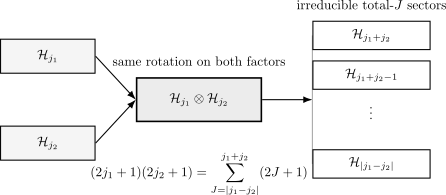
The tensor product is the composite Hilbert space. Under the diagonal rotation action it decomposes into irreducible sectors from $J=|j_1-j_2|$ through $J=j_1+j_2$.

For three or more factors, the same total $J$ can occur with multiplicity. Extra intermediate-coupling labels are then needed to distinguish equivalent irreducible sectors.

Coupled and Uncoupled Bases

The uncoupled basis is

$$|j_1,m_1\rangle |j_2,m_2\rangle.$$

It diagonalizes

$$J_1^2, \quad J_{1z}, \quad J_2^2, \quad J_{2z}.$$

The coupled basis is

$$|j_1,j_2;J,M\rangle.$$

It diagonalizes

$$J_1^2, \quad J_2^2, \quad J^2, \quad J_z.$$

Both bases are orthonormal and complete in the same fixed-$j_1,j_2$ tensor-product space. The useful basis is determined by the observables and Hamiltonian:

Structure in the problem	Usually natural basis
separate fields or measurements of $J_{1z}$ and $J_{2z}$	uncoupled
rotationally invariant interaction $f(\mathbf J_1\cdot\mathbf J_2)$	coupled
strong external field overwhelming internal coupling	often uncoupled or partially uncoupled
internal scalar coupling dominating weak fields	coupled

The magnetic labels satisfy

$$M=m_1+m_2.$$

This relation is exact because $J_z$ is additive. It is not a vector-model approximation.

Clebsch–Gordan Coefficients

Clebsch–Gordan coefficients are the unitary change-of-basis amplitudes:

$$\begin{aligned} |j_1,j_2;J,M\rangle &= \sum_{m_1,m_2} C^{JM}_{j_1m_1,j_2m_2} \\ &\quad\times |j_1,m_1\rangle |j_2,m_2\rangle. \end{aligned}$$

The coefficient is the overlap

$$C^{JM}_{j_1m_1,j_2m_2} = \langle j_1,m_1;j_2,m_2|J,M\rangle.$$

Before consulting a table, apply the zero tests:

$$M=m_1+m_2,$$ $$|j_1-j_2| \leq J\leq j_1+j_2,$$

and all projection labels must lie in their allowed ranges. Surviving coefficients obey normalization and orthogonality because the basis change is unitary.

For small angular momenta, a constructive method is often clearer than a table:

1. Start from the highest-weight product state for $J=j_1+j_2$.
2. Apply $J_-=J_{1-}+J_{2-}$ and normalize.
3. Use orthogonality to find states with the same $M$ but smaller $J$.
4. Continue lowering within each multiplet.

This volume uses the Condon–Shortley phase convention. Coefficient signs depend on state-phase conventions, so a numerical table is incomplete unless it states its convention and the ordering of $j_1,j_2$.

Interchanging the factors gives

$$\begin{aligned} &\langle j_2,m_2;j_1,m_1|J,M\rangle \\ &\quad= (-1)^{j_1+j_2-J} \langle j_1,m_1;j_2,m_2|J,M\rangle. \end{aligned}$$

The exponent is an integer for an allowed coupling. This phase relation is why factor order cannot be ignored even though the two tensor-product spaces are naturally isomorphic.

Two Spin-One-Half Systems

For two spin-$1/2$ factors,

$$\frac12\otimes\frac12 = 1\oplus0.$$

The four-dimensional product space becomes a three-dimensional triplet plus a one-dimensional singlet. In the standard phase convention,

$$|1,1\rangle = |\uparrow\uparrow\rangle,$$ $$|1,0\rangle = \frac{1}{\sqrt2} \left( |\uparrow\downarrow\rangle + |\downarrow\uparrow\rangle \right),$$ $$|1,-1\rangle = |\downarrow\downarrow\rangle,$$

and

$$|0,0\rangle = \frac{1}{\sqrt2} \left( |\uparrow\downarrow\rangle - |\downarrow\uparrow\rangle \right).$$

The relative sign distinguishes the $M=0$ triplet from the singlet. An overall phase multiplying either complete state would not change its ray.

The inverse relations are equally useful:

$$|\uparrow\downarrow\rangle = \frac{|1,0\rangle+|0,0\rangle}{\sqrt2},$$ $$|\downarrow\uparrow\rangle = \frac{|1,0\rangle-|0,0\rangle}{\sqrt2}.$$

Thus a product state with total projection $M=0$ need not have definite total spin. Measuring $S^2$ in $|\uparrow\downarrow\rangle$ gives the triplet and singlet sectors with equal probability.

Singlet and Triplet as Symmetry Sectors

Under joint rotations, the triplet states mix among themselves as a spin-$1$ multiplet. The singlet is annihilated by every component of total spin:

$$\mathbf S|0,0\rangle=0.$$

Therefore

$$U(R)|0,0\rangle = |0,0\rangle$$

for every joint spin rotation. The singlet is a rotational scalar; the triplet carries the vector representation.

The scalar product

$$\mathbf S_1\cdot\mathbf S_2 = \frac12 \left( S^2-S_1^2-S_2^2 \right)$$

has eigenvalues

$$\frac{\hbar^2}{4} \quad\text{on the triplet},$$

and

$$-\frac{3\hbar^2}{4} \quad\text{on the singlet}.$$

Consequently, the sector projectors can be written without choosing an axis:

$$P_{\mathrm{triplet}} = \frac34 I + \frac{\mathbf S_1\cdot\mathbf S_2}{\hbar^2},$$ $$P_{\mathrm{singlet}} = \frac14 I - \frac{\mathbf S_1\cdot\mathbf S_2}{\hbar^2}.$$

These formulas expose the representation sectors directly. The singlet’s entanglement and Bell-correlation roles belong to Composite-Systems Singlet and Triplet States; here the canonical point is their transformation under rotations.

Scalar Couplings Become Simple in the Coupled Basis

For any two angular momenta,

$$\mathbf J_1\cdot\mathbf J_2 = \frac12 \left( J^2-J_1^2-J_2^2 \right).$$

On a coupled state this becomes the number

$$\begin{aligned} \mathbf J_1\cdot\mathbf J_2 \longrightarrow \frac{\hbar^2}{2} \bigl[ &J(J+1) \\ &\quad-j_1(j_1+1) \\ &\quad-j_2(j_2+1) \bigr]. \end{aligned}$$

Therefore a rotationally invariant Hamiltonian

$$H=A\,\mathbf J_1\cdot\mathbf J_2$$

is diagonal in the coupled basis. The coefficient $A$ contains system-dependent dynamics; angular momentum addition supplies the universal eigenvalue pattern.

This is the recurring strategy:

1. identify the conserved total angular momentum;
2. rewrite scalar products using Casimir operators;
3. evaluate the Casimir eigenvalues;
4. leave radial integrals or material-specific coefficients to the system’s canonical page.

The method explains exchange-model singlet–triplet splittings, orbital-spin splittings, and hyperfine multiplets without diagonalizing every matrix element in the uncoupled basis.

Adding Orbital and Spin Angular Momentum

A particle with orbital angular momentum $\mathbf L$ and spin $\mathbf S$ has total rotation generator

$$\mathbf J=\mathbf L+\mathbf S.$$

The uncoupled basis is

$$|n,\ell,m_\ell\rangle |s,m_s\rangle,$$

while the coupled basis is

$$|n,\ell,s;j,m_j\rangle.$$

The magnetic labels satisfy

$$m_j=m_\ell+m_s.$$

For spin $s=1/2$ and $\ell>0$,

$$j=\ell-\frac12, \qquad j=\ell+\frac12.$$

When $\ell=0$, only $j=1/2$ occurs. The dimensions provide a quick check:

$$2(2\ell+1) = 2\ell+(2\ell+2).$$

The angular-spin wavefunction can be packaged into a spinor spherical harmonic,

$$\begin{aligned} \Omega_{\ell jm_j}(\theta,\phi) &= \sum_{m_\ell,m_s} \langle\ell,m_\ell; \tfrac12,m_s|j,m_j\rangle \\ &\quad\times Y_\ell^{m_\ell}(\theta,\phi) \chi_{m_s}. \end{aligned}$$

Spin does not alter the orbital parity, so this state has parity $(-1)^\ell$. The total label $j$ alone does not determine parity because the same $j$ can arise from different $\ell$ values.

Spin–Orbit Coupling

In a central-potential model, spin–orbit coupling has the angular form

$$H_{\mathrm{SO}} = \xi(r)\, \mathbf L\cdot\mathbf S.$$

It is a scalar under rotations generated by $\mathbf J=\mathbf L+\mathbf S$. The identity

$$\mathbf L\cdot\mathbf S = \frac12 \left( J^2-L^2-S^2 \right)$$

makes the coupled basis diagonal. Its angular eigenvalue is

$$\begin{aligned} \mathbf L\cdot\mathbf S \longrightarrow \frac{\hbar^2}{2} \bigl[ &j(j+1) \\ &-\ell(\ell+1) -s(s+1) \bigr]. \end{aligned}$$

For $s=1/2$,

$$\mathbf L\cdot\mathbf S = \frac{\hbar^2\ell}{2} \quad \text{when }j=\ell+\frac12,$$

and

$$\mathbf L\cdot\mathbf S = -\frac{\hbar^2(\ell+1)}{2} \quad \text{when }j=\ell-\frac12.$$

The radial coefficient $\xi(r)$, its expectation value, and the microscopic origin of the interaction are not fixed by angular momentum algebra. Atomic fine structure, relativistic derivations, and solid-state spin–orbit mechanisms therefore remain separate canonical topics.

Coupling Schemes Follow the Hamiltonian Hierarchy

A coupling scheme specifies which angular momenta are combined first and which intermediate Casimirs are used as labels. It is a basis choice, not a different Hilbert space or a new law of addition.

Scheme	First couplings	Later coupling	Typical useful regime
LS or Russell–Saunders	all $\mathbf l_i$ to $\mathbf L$; all $\mathbf s_i$ to $\mathbf S$	$\mathbf J=\mathbf L+\mathbf S$	spin-independent interactions dominate individual spin–orbit terms
jj	each $\mathbf j_i=\mathbf l_i+\mathbf s_i$	$\mathbf J=\sum_i\mathbf j_i$	individual spin–orbit interactions are strong
hyperfine	electronic $\mathbf J$ and nuclear $\mathbf I$	$\mathbf F=\mathbf J+\mathbf I$	resolved hyperfine structure in sufficiently weak fields
molecular	electronic, spin, and rotational angular momenta in a chosen order	total molecular angular momentum	hierarchy depends on the molecular Hamiltonian

For example, LS coupling uses term labels schematically written

$${}^{2S+1}L_J.$$

Hyperfine coupling gives

$$F=|J-I|, |J-I|+1, \ldots, J+I.$$

When competing Hamiltonian terms have comparable size, neither limiting scheme may provide exact labels. Intermediate coupling means diagonalizing within a symmetry sector and treating labels such as $L$ and $S$ as approximate according to the actual mixing.

The practical rule is to diagonalize the dominant interaction first. A label is good only if its operator commutes with the relevant Hamiltonian, or approximately good only when the symmetry-breaking terms are controlled.

Recoupling and Wigner Symbols

For three angular momenta, one may first form

$$\mathbf J_{12}=\mathbf J_1+\mathbf J_2$$

and use

$$|(j_1j_2)j_{12},j_3;J,M\rangle,$$

or first form

$$\mathbf J_{23}=\mathbf J_2+\mathbf J_3$$

and use

$$|j_1,(j_2j_3)j_{23};J,M\rangle.$$

Both bases diagonalize $J^2$ and $J_z$, but they diagonalize different intermediate Casimirs. The unitary transformation between them is encoded by a Wigner $6j$ symbol.

The hierarchy of symbols is:

Symbol	Main role
Wigner $3j$	writes Clebsch–Gordan data in a more symmetric notation
Wigner $6j$	changes the binary coupling order of three angular momenta
Wigner $9j$	compares common pairwise coupling schemes for four angular momenta

With the convention used here, the $3j$ relation is

$$\begin{aligned} &\langle j_1,m_1;j_2,m_2|J,M\rangle \\ &\quad= (-1)^{j_1-j_2+M} \sqrt{2J+1} \\ &\qquad\times \begin{pmatrix} j_1&j_2&J\\ m_1&m_2&-M \end{pmatrix}. \end{aligned}$$

Wigner symbols do not add new dynamics. They package basis transformations and symmetry constraints. Their phase and normalization conventions must be checked just as carefully as Clebsch–Gordan tables.

Exchange Symmetry Preview

For two identical spin-$s$ factors, a coupled spin state has exchange parity

$$P_{12}|s,s;S,M\rangle = (-1)^{2s-S} |s,s;S,M\rangle.$$

For two spin-$1/2$ systems, the triplet is symmetric and the singlet is antisymmetric. For identical fermions, the total state must be antisymmetric; therefore a symmetric spin part requires an antisymmetric spatial part, and an antisymmetric spin part requires a symmetric spatial part.

Spin sector for two electrons	Spin exchange parity	Required spatial parity
triplet, $S=1$	$+1$	$-1$
singlet, $S=0$	$-1$	$+1$

This table is a consequence of combining angular momentum with the symmetrization postulate. It is not a derivation of the spin–statistics connection, and the labels “bosonic” or “fermionic” should not be attached to the spin sectors themselves. The full rule applies to every degree of freedom in the total state.

A Reliable Workflow

For a new angular-momentum addition problem:

1. List the factors. Record each $j_a$, its Hilbert-space dimension, and the operators acting on it.
2. Write the tensor product. Do not replace the composite space by a direct sum before identifying the joint rotation action.
3. Define the total generator. Include identity factors when operator placement could be ambiguous.
4. Apply the triangle rule. List the allowed total-$J$ values and check the dimension sum.
5. Choose a basis from the Hamiltonian. Decide which complete commuting set is natural before expanding states.
6. Apply zero tests. Use $M=\sum_a m_a$ and triangle conditions before consulting coefficient tables.
7. Declare conventions. State the Clebsch–Gordan phase convention and ordering of factors.
8. Rewrite scalar products with Casimirs. This often diagonalizes the interaction immediately.
9. Separate symmetry from dynamics. Angular coefficients are universal; radial integrals, coupling strengths, and material parameters are not.
10. For three or more factors, record intermediate labels. Different coupling orders are related by recoupling coefficients rather than by new physics.

Chapter Map

Read this page	When the question is
Tensor Product Representations	Why does a composite rotation representation decompose into total-$J$ sectors?
Total Angular Momentum	What operator generates a joint rotation?
Coupled and Uncoupled Bases	Which observables are diagonal in each basis?
Two Spin-1/2 Particles	How is the first nontrivial decomposition constructed?
Singlet and Triplet States	What do the scalar and vector sectors mean physically?
Clebsch–Gordan Coefficients	How are coupled and uncoupled states related numerically?
Clebsch–Gordan Tables and Conventions	How can a coefficient be read without losing a sign or normalization?
Angular Momentum Coupling Schemes	Which coupling order matches a given hierarchy of interactions?
Spin–Orbit Coupling	Why does the $J^2$ identity diagonalize $\mathbf L\cdot\mathbf S$?
Addition of Orbital and Spin Angular Momentum	How are one-particle spinor wavefunctions labeled?
Recoupling and Wigner Symbols	How are different coupling orders compared?
Identical Particles and Exchange Symmetry Preview	How does coupled-spin symmetry constrain the spatial factor?

Reading Paths

First complete pass

1. Tensor Product Representations
2. Total Angular Momentum
3. Coupled and Uncoupled Bases
4. Two Spin-1/2 Particles
5. Clebsch–Gordan Coefficients

Atomic and spectroscopic route

1. Addition of Orbital and Spin Angular Momentum
2. Spin–Orbit Coupling
3. Angular Momentum Coupling Schemes
4. Tensor Operators and Selection Rules
5. Wigner–Eckart Theorem

Several-angular-momentum route

1. Clebsch–Gordan Tables and Conventions
2. Recoupling and Wigner Symbols
3. Wigner Symbols Quick Reference

Composite-system route

1. Singlet and Triplet States
2. Identical Particles and Exchange Symmetry Preview
3. Spin and Spatial Wavefunctions

Distinctions Worth Keeping

Do not conflate	Why
tensor product and direct sum	the tensor product is the composite space; the direct sum is its irreducible decomposition under joint rotations
adding generators and adding quantum numbers	operators add componentwise, while allowed total $J$ values follow the triangle rule
product state and coupled state	a product state has definite subsystem projections but usually indefinite total $J$
basis transformation and physical interaction	Clebsch–Gordan coefficients change coordinates; the Hamiltonian determines energies and dynamics
total $M$ and total $J$	$M=\sum m_a$ is additive, while $J$ is constrained by representation coupling
phase convention and measurable phase	table signs depend on basis conventions, but consistent complete amplitudes give convention-independent predictions
coupling order and physical system	recoupling changes the basis, not the underlying state space
spin exchange symmetry and particle statistics	the full identical-particle state, not only the spin factor, obeys the symmetrization rule

Common Mistakes

• Reading $j_1\otimes j_2=J_1\oplus J_2\oplus\cdots$ as ordinary arithmetic.
• Omitting identity operators when subsystem operator placement is ambiguous.
• Assuming $|j_1,m_1\rangle|j_2,m_2\rangle$ is automatically an eigenstate of $J^2$.
• Forgetting either the triangle rule or $M=m_1+m_2$ before table lookup.
• Mixing Condon–Shortley coefficients with a table using a different phase convention.
• Interchanging $j_1$ and $j_2$ without the corresponding phase factor.
• Calling the $M=0$ triplet a singlet because its total projection vanishes.
• Treating LS and jj coupling as exact universal classifications rather than limiting schemes adapted to a Hamiltonian hierarchy.
• Using a Wigner $3j$ number as a Clebsch–Gordan coefficient without the conversion factor.
• Applying spin exchange parity without constructing the full spatial-spin state.

Cross-Links

• Spin and Spinors
• Angular Momentum Algebra
• Tensor Products
• Complete Sets of Commuting Observables
• Tensor Product Representations in the Mathematical Toolkit
• Clebsch–Gordan Coefficients in the Mathematical Toolkit
• Clebsch–Gordan Quick Reference
• Angular Momentum Problems
• Spin and Spatial Wavefunctions
• Tensor Operators and Selection Rules
• Wigner–Eckart Theorem

References

• J. J. Sakurai and J. Napolitano, Modern Quantum Mechanics, 3rd ed., Cambridge University Press, 2020.
• R. Shankar, Principles of Quantum Mechanics, 2nd ed., Springer, 1994.
• C. Cohen-Tannoudji, B. Diu, and F. Laloë, Quantum Mechanics, Wiley, 1977.
• A. R. Edmonds, Angular Momentum in Quantum Mechanics, Princeton University Press, 1957.
• D. M. Brink and G. R. Satchler, Angular Momentum, 3rd ed., Oxford University Press, 1993.
• D. A. Varshalovich, A. N. Moskalev, and V. K. Khersonskii, Quantum Theory of Angular Momentum, World Scientific, 1988.
• R. N. Zare, Angular Momentum: Understanding Spatial Aspects in Chemistry and Physics, Wiley, 1988.

Exercises

1. Couple $j_1=1$ and $j_2=3/2$. List the allowed total $J$ values and verify the dimension identity.

Solution

The triangle rule gives

$$J = \frac12, \frac32, \frac52.$$

The product-space dimension is

$$(2j_1+1)(2j_2+1) = 3\cdot4 = 12.$$

The irreducible-sector dimensions are

$$2J+1=2,4,6,$$

and $2+4+6=12$ as required.

2. Express $|\uparrow\downarrow\rangle$ in the coupled basis. What are the probabilities for total spin $S=1$ and $S=0$? Also state its exchange behavior.

Solution

Using the standard singlet and triplet states,

$$|\uparrow\downarrow\rangle = \frac{|1,0\rangle+|0,0\rangle}{\sqrt2}.$$

The two total-spin outcomes therefore each have probability $1/2$. The product state is not an eigenstate of exchange:

$$P_{12}|\uparrow\downarrow\rangle = |\downarrow\uparrow\rangle.$$

Its symmetric and antisymmetric components are precisely the triplet and singlet terms in the coupled expansion.

3. Two spin-$1/2$ systems interact through

$$H=A\,\mathbf S_1\cdot\mathbf S_2.$$

Find the singlet and triplet energies, their degeneracies, and the level separation.

Solution

The scalar product has eigenvalue $\hbar^2/4$ in the triplet and $-3\hbar^2/4$ in the singlet. Hence

$$\begin{gathered} E_{\mathrm{triplet}} = \frac{A\hbar^2}{4}, \\ g_{\mathrm{triplet}}=3, \end{gathered}$$

and

$$\begin{gathered} E_{\mathrm{singlet}} = -\frac{3A\hbar^2}{4}, \\ g_{\mathrm{singlet}}=1. \end{gathered}$$

Their signed difference is

$$E_{\mathrm{triplet}}-E_{\mathrm{singlet}} = A\hbar^2.$$

For $A>0$ the singlet lies lower; for $A<0$ the triplet lies lower.

4. Add orbital angular momentum $\ell=2$ to spin $s=1/2$. Find the allowed $j$ values, check the dimensions, and evaluate $\mathbf L\cdot\mathbf S$ in each sector.

Solution

The allowed total angular momenta are

$$j=\frac52, \qquad j=\frac32.$$

Their dimensions are $6$ and $4$, matching

$$(2\ell+1)(2s+1)=5\cdot2=10.$$

For $j=\ell+1/2=5/2$,

$$\mathbf L\cdot\mathbf S = \frac{\hbar^2\ell}{2} = \hbar^2.$$

For $j=\ell-1/2=3/2$,

$$\mathbf L\cdot\mathbf S = -\frac{\hbar^2(\ell+1)}{2} = -\frac{3\hbar^2}{2}.$$

5. Decompose the representation of three spin-$1/2$ systems and explain why an intermediate coupling label is needed.

Solution

First couple two spins:

$$\frac12\otimes\frac12 = 1\oplus0.$$

Then add the third spin:

$$\begin{aligned} (1\oplus0)\otimes\frac12 &= \left( \frac32\oplus\frac12 \right) \oplus \frac12 \\ &= \frac32 \oplus \frac12 \oplus \frac12. \end{aligned}$$

The dimensions check:

$$2^3=8=4+2+2.$$

Total $J=1/2$ occurs twice. A label such as $j_{12}=0$ or $j_{12}=1$ distinguishes the two copies in the coupling scheme that combines spins $1$ and $2$ first. Changing to a basis labeled by $j_{23}$ is a recoupling transformation governed by a Wigner $6j$ symbol.