Precision Measurement and Metrology

Precision measurement uses a physical system to estimate a quantity with a stated uncertainty. Metrology adds the discipline needed to make that estimate comparable across instruments, laboratories, places, and times: an explicit measurand, a calibrated measurement model, traceability, uncertainty propagation, stability analysis, and tests for unrecognized bias.

Atomic, molecular, and optical systems are unusually powerful metrological resources because quantum mechanics supplies reproducible energy differences. For two stationary states,

$$h\nu_0 = E_e-E_g.$$

The transition frequency $\nu_0$ can be interrogated repeatedly, compared with an oscillator, and connected by frequency division or a frequency comb to electronic counters. The same logic extends beyond clocks. A magnetic field produces a Zeeman shift, an acceleration produces an interferometer phase, an electric dipole moment produces an energy shift, and a change in a dimensionless constant changes a frequency ratio.

The quantum transition is not an incorruptible number displayed by nature. The measured resonance is shifted by fields, motion, collisions, probing, gravity, and servo dynamics. It is broadened by finite interrogation, decoherence, oscillator noise, and inhomogeneity. Detection adds projection noise and technical noise. Precision AMO metrology is the art of exploiting the reproducibility of quantum structure while measuring every relevant way the apparatus perturbs it.

Canonical Scope

Precision Spectroscopy owns line-center estimation, narrow-transition physics, correction budgets, frequency ratios, and the spectroscopy-to-new-physics workflow. Ramsey Interferometry owns the separated-pulse derivation, finite-pulse fringe, discriminator, clock cycle, and local-oscillator noise. Frequency Combs owns comb-tooth frequencies, carrier-envelope offset, self-referencing, transfer oscillators, and optical frequency division.

Quantum Sensing owns the general parameter-estimation, Fisher-information, backaction, decoherence, and noise-spectroscopy framework. Fisher Information owns the classical score, Cramér–Rao bound, additivity, and multiparameter Fisher matrix. Atom Interferometry owns light-pulse beam splitters, inertial phase derivations, sensitivity functions, wave-packet closure, and platform calibration. Squeezed Light owns optical quadrature squeezing, homodyne verification, loss, and interferometric readout.

This chapter overview owns:

• the complete AMO metrology chain from measurand to reported result;
• the distinction among resolution, precision, stability, bias, and measurement uncertainty;
• frequency and phase as universal AMO readout coordinates;
• a generic passive-reference and sensor loop;
• a covariance-aware systematic-correction ledger;
• quantum projection noise and the independent-particle scaling;
• an operational preview of spin squeezing and quantum enhancement;
• a map of clocks, field sensors, inertial sensors, constants, and fundamental tests; and
• the evidence required for a traceable and reproducible claim.

The pages that follow own the detailed architectures and uncertainty budgets for individual classes of instrument.

Metrological Language

Measurand and measurement model

The measurand is the quantity intended to be measured. It must be specified closely enough that different implementations refer to the same quantity. “The transition frequency” is often incomplete. A clock measurand might instead be:

the unperturbed frequency of a specified transition in a specified isotope, for an atom at rest, in a declared reference frame, with stated field and environmental conventions.

A measurement model relates the output quantity $Y$ to input quantities:

$$Y = f \left( X_1,X_2,\ldots,X_n \right).$$

The inputs can include raw observations, calibration constants, environmental parameters, theoretical coefficients, and corrections. A reported result is therefore not merely an average of detector readings. It is an inference through $f$.

Indication, correction, and result

For a frequency measurement, write a representative model as

$$\nu_{\mathrm{obs}} = \nu_0 + \sum_i \Delta\nu_i + \epsilon_{\mathrm{stat}},$$

where $\nu_0$ is the target unperturbed frequency, $\Delta\nu_i$ are systematic shifts, and $\epsilon_{\mathrm{stat}}$ represents zero-mean statistical fluctuation in the stated averaging protocol. The corrected estimate is

$$\widehat{\nu}_0 = \overline{\nu}_{\mathrm{obs}} - \sum_i \widehat{\Delta\nu}_i.$$

Some laboratories tabulate corrections to add rather than shifts to subtract. Both conventions are valid, but the sign convention must be stated and checked with a synthetic example.

Precision, stability, and uncertainty

These words answer different questions:

Term	Question	Typical evidence
Resolution	What is the smallest display increment or distinguishable feature?	digitization, linewidth, response curve
Repeatability	How closely do repeated results agree under fixed conditions?	repeated trials
Precision	How dispersed are repeated estimates?	standard deviation or interval
Stability	How do frequency or phase fluctuations depend on averaging time?	Allan-family statistics, spectra
Bias	How far is an estimator displaced in expectation?	calibration, reversal, comparison
Measurement uncertainty	What range of values is reasonably attributable to the measurand under the model?	propagated statistical and systematic evaluation
Traceability	Through what documented calibration chain is the result related to a reference?	comparison records and uncertainty chain

Stability does not establish that a frequency is correct. A quiet oscillator can have a fixed offset. Conversely, a well-evaluated reference can have a large short-term instability and still yield an unbiased long-term result.

Accuracy is not a number by itself

In formal metrology, measurement accuracy is a qualitative closeness concept rather than a quantity with its own numerical value. Experimental papers often use “accuracy” informally for small systematic uncertainty. Clearer reporting separates:

$$\text{measured offset}, \qquad \text{statistical uncertainty}, \qquad \text{systematic uncertainty}, \qquad \text{total uncertainty}.$$

The AMO Metrology Chain

Seven linked stages

A complete instrument can be organized into seven stages:

1. Define the measurand. State the quantity, system, reference frame, operating conditions, and averaging interval.
2. Transduce it into quantum dynamics. Specify how the quantity changes an energy, rate, force, phase, or transition probability.
3. Prepare and interrogate the probe. Define states, controls, timing, oscillator phase, and environment.
4. Measure an outcome. Specify the POVM or detector model, assignment errors, loss, and dead time.
5. Estimate a parameter. State the likelihood, estimator, priors if used, and treatment of nuisance parameters.
6. Correct systematic effects. Measure sensitivity coefficients, environmental inputs, correlations, and model uncertainty.
7. Validate and compare. Use reversals, scaling tests, independent sensors, ratios, blind offsets, and interlaboratory comparisons.

Failure at any stage can dominate the final result even when the quantum transition is extremely narrow.

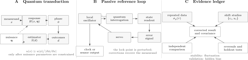
Three views of an AMO measurement. A: the measurand $x$ changes a Hamiltonian or phase and is inferred from outcomes through an estimator. B: a passive frequency standard compares a local oscillator with a quantum transition and feeds an error signal back to the oscillator. C: stability data and systematic-effect studies are distinct evidence streams; comparison and holdout tests constrain effects that the nominal model may have missed.

Transduction coefficient

Suppose a quantity $x$ changes a measured frequency. Near an operating point,

$$\delta\nu \simeq \left. \frac{\partial\nu}{\partial x} \right|_{x_0} \delta x.$$

Define the dimensional transduction coefficient

$$k_x = \frac{\partial\nu}{\partial x}.$$

Then a frequency-estimation uncertainty $u(\nu)$ corresponds, in the linear regime, to

$$u(x) \simeq \frac{u(\nu)}{|k_x|}.$$

Large $|k_x|$ is useful only if nuisance quantities do not produce indistinguishable shifts. Selectivity and independent controls matter as much as raw response.

For a dimensionless parameter $X$, the logarithmic sensitivity coefficient

$$K_X = \frac{\partial\ln\nu}{\partial\ln X}$$

gives

$$\frac{\delta\nu}{\nu} \simeq K_X \frac{\delta X}{X}.$$

Frequency-ratio comparisons involve differences of sensitivity coefficients and remove dependence on a unit realization.

Calibration is an experiment

If the shift model is

$$\Delta\nu_B = \beta B^2,$$

then neither $\beta$ nor $B$ should be treated as an unexamined label. $\beta$ may come from theory, an auxiliary measurement, or an in situ field scan. $B$ may be inferred from a magnetically sensitive transition rather than a remote probe. The calibration procedure has its own transfer function, gradients, time dependence, and uncertainty.

Why Quantum Systems Make References

Identical particles and reproducible structure

Atoms of one isotope are not manufactured artifacts with individually different dimensions. Within a specified internal state and environment, they realize the same quantum Hamiltonian. This supports reproducibility across apparatus and laboratories.

The statement has limits. Isotope composition, hyperfine state, motional state, local fields, collisions, trap light, and relativistic potential all matter. Identical bare particles do not imply identical perturbed frequencies.

Narrow transitions and quality factor

A transition with ordinary frequency $\nu_0$ and observed linewidth $\Delta\nu$ has quality factor

$$Q = \frac{\nu_0}{\Delta\nu}.$$

For a fixed signal-to-noise ratio, larger $Q$ usually permits finer fractional discrimination. Optical frequencies also provide a larger phase accumulation per unit fractional detuning than microwave frequencies:

$$\phi = 2\pi \int_0^T \delta\nu(t)\,dt.$$

A narrow natural linewidth is not enough. The local oscillator, probe time, coherence, state preparation, and systematic shifts determine the usable line.

Long coherence and controlled isolation

Useful references suppress or characterize environmental coupling while retaining controlled preparation and readout. Examples include:

• hyperfine “clock” states with canceled first-order Zeeman sensitivity;
• forbidden optical transitions with long excited-state lifetimes;
• ions confined near the Lamb–Dicke regime;
• neutral atoms trapped at a magic wavelength;
• molecular states with enhanced sensitivity to symmetry-violating interactions; and
• spin ensembles with long transverse coherence.

Isolation and sensitivity compete. A sensor must couple strongly enough to the desired quantity while rejecting or separately measuring nuisance couplings.

Ratios are especially powerful

An absolute frequency measurement compares against a realization of the unit hertz. A ratio

$$R = \frac{\nu_A}{\nu_B}$$

is dimensionless. Optical combs can compare distant optical frequencies coherently, and many oscillator fluctuations can cancel in synchronous or transfer-oscillator schemes. Repeated ratio measurements are central to clock validation and searches for changes in dimensionless constants.

Frequency as a Measurable Quantity

Phase is the immediate observable

Frequency is inferred from accumulated phase. For an oscillator

$$V(t) = V_0 \cos \left[ 2\pi\nu_0t+\phi(t) \right],$$

the instantaneous frequency deviation is

$$\delta\nu(t) = \frac{1}{2\pi} \frac{d\phi}{dt}.$$

No finite-duration experiment measures an instantaneous mathematical frequency. It estimates an average phase slope over a specified interval and bandwidth.

Fractional frequency

For a nominal reference frequency $\nu_0$, define

$$y(t) = \frac{\nu(t)-\nu_0}{\nu_0}.$$

Fractional frequency makes microwave and optical systems comparable and connects directly to relativistic and constant-variation signals. An average over an interval $\tau$ is

$$\overline y_k(\tau) = \frac{1}{\tau} \int_{t_k}^{t_k+\tau} y(t)\,dt.$$

The associated accumulated time or phase error depends on the integral of $y(t)$, not just its pointwise value.

Passive and active references

In a passive atomic standard, an external local oscillator interrogates the atoms. The atoms provide a discriminator; a servo corrects the oscillator. Most primary and optical clocks use this architecture.

In an active standard, stimulated emission from the atomic medium directly sustains an oscillator. Hydrogen masers are a familiar example. The distinction concerns how the output is generated, not whether quantum states are involved.

Passive-reference loop

Let $\nu_{\mathrm{LO}}$ be the local-oscillator frequency and $\nu_a$ the perturbed atomic resonance. An interrogation produces an error signal

$$e_k \simeq D \left( \nu_{\mathrm{LO},k}-\nu_{a,k} \right) + n_k$$

near the lock point, where $D$ is the discriminator slope and $n_k$ is measurement noise. A simple digital integrator updates

$$\nu_{\mathrm{LO},k+1} = \nu_{\mathrm{LO},k} - g e_k.$$

The loop tracks the perturbed atomic resonance, not automatically the unperturbed measurand $\nu_0$. Corrections for Zeeman, Stark, collision, motion, gravity, probe, and servo effects remain necessary.

Current SI second

As of the review date of this page, the SI second remains defined by fixing the unperturbed ground-state hyperfine transition frequency of $^{133}\mathrm{Cs}$ to exactly

$$\Delta\nu_{\mathrm{Cs}} = 9\,192\,631\,770\ \mathrm{Hz}.$$

The Consultative Committee for Time and Frequency is developing a possible future redefinition based on optical-frequency standards. The BIPM roadmap describes a process and criteria, not an already enacted definition. Pages that discuss the SI must distinguish the current legal definition from secondary representations and from candidate future transitions.

Stability

Allan variance

For adjacent fractional-frequency averages of duration $\tau$, the two-sample Allan variance is

$$\sigma_y^2(\tau) = \frac{1}{2} \left\langle \left[ \overline y_{k+1}(\tau) - \overline y_k(\tau) \right]^2 \right\rangle.$$

The Allan deviation is

$$\sigma_y(\tau) = \sqrt{\sigma_y^2(\tau)}.$$

It is a function of averaging time. A statement such as “the stability is $10^{-16}$” is incomplete without $\tau$, the statistic variant, sampling protocol, uncertainty, and treatment of drift or dead time.

For $M$ adjacent samples,

$$\widehat{\sigma}_y^2(\tau) = \frac{1}{ 2(M-1) } \sum_{k=1}^{M-1} \left( \overline y_{k+1} - \overline y_k \right)^2.$$

Overlapping Allan deviation uses more of a phase record and has different degrees of freedom. Modified Allan, Hadamard, and total deviations answer related but distinct questions. The chosen statistic should match the noise and data structure.

White-frequency scaling

For uncorrelated cycle-to-cycle frequency estimates,

$$\sigma_y(\tau) \propto \tau^{-1/2}.$$

Flicker noise, random walk, environmental cycles, drift, and servo dynamics produce different slopes or floors. A fitted power law over a short range does not identify a unique microscopic noise source.

Dead time and oscillator aliasing

If atoms are interrogated only during part of each cycle, local-oscillator noise during dead time is not observed continuously. Periodic sampling can alias oscillator noise into the measurement band, producing the Dick effect. Increasing atom number does not suppress this classical oscillator contribution. Higher duty cycle, synchronous comparison, better local oscillators, and zero-dead-time architectures address it.

Comparison is the observable

A single oscillator cannot reveal its own absolute instability. Stability is inferred from a comparison:

$$y_{AB}(t) = y_A(t)-y_B(t).$$

Separating individual contributions requires assumptions, a third reference, cross-correlation, or a known noise hierarchy. Common-mode environment and shared oscillators can make a comparison look quieter than either independent system.

Systematic Shifts

Generic correction ledger

For a clock or frequency sensor, a useful ledger is

$$\frac{\widehat{\nu}_0-\nu_{\mathrm{ref}}}{\nu_0} = y_{\mathrm{obs}} + \sum_i c_i,$$

where $c_i$ are fractional corrections to add under this convention. Each entry should include:

• physical mechanism;
• mathematical model;
• measured operating parameter;
• correction and sign;
• standard uncertainty;
• sensitivity to analysis choices;
• covariance with other entries; and
• validation or reversal test.

The total is not more trustworthy than the least-tested material entry.

Representative mechanisms

Mechanism	Typical dependence	Diagnostic
Linear Zeeman	$m_F B$	reverse $m_F$, field scan, magnetically sensitive line
Quadratic Zeeman	$\beta B^2$	vary field magnitude, independent field monitor
DC Stark	scalar, vector, and tensor polarizability terms	reverse electric field, polarization and orientation scan
Blackbody radiation	dynamic polarizability and thermal spectrum	temperature map, emissivity and view-factor model
Probe light	intensity, detuning, pulse area, line shape	interleaved intensity and duration scan
Trap or lattice light	differential polarizability, multipolar terms	wavelength and depth scan
Motion	first- and second-order Doppler, recoil, time dilation	sideband thermometry, velocity reversal
Collisions	density and state correlations	atom-number or density extrapolation
Line pulling	neighboring components and asymmetric response	resolve components, vary preparation and fit model
Servo error	discriminator offset, drift, loop delay	reverse modulation, alter gain and cycle
Gravity	gravitational potential	surveyed height and potential model

The relevant list depends on the platform. A correction budget copied from a different species or apparatus is not an evaluation.

Covariance-aware propagation

For

$$Y = f(\mathbf X),$$

the first-order combined variance is

$$u_c^2(Y) = \sum_{i,j} \frac{\partial f}{\partial X_i} \frac{\partial f}{\partial X_j} \operatorname{Cov} \left( X_i,X_j \right).$$

Equivalently,

$$u_c^2(Y) = \mathbf g^{\mathsf T} \mathbf C \mathbf g,$$

where $g_i=\partial f/\partial X_i$ and $\mathbf C$ is the covariance matrix. Adding standard uncertainties in quadrature assumes the relevant covariances vanish.

Worked correction-budget audit

Suppose a fractional comparison gives

$$y_{\mathrm{obs}} = 7.40\times10^{-16}.$$

Under the correction-to-add convention, let

$$\begin{array}{c|c|c} \text{effect} & c_i/(10^{-16}) & u_i/(10^{-16}) \\ \hline \text{blackbody} & -5.20 & 0.40 \\ \text{quadratic Zeeman} & +0.60 & 0.20 \\ \text{density} & -0.30 & 0.30 \end{array}$$

Then

$$\widehat y = \left( 7.40-5.20+0.60-0.30 \right) \times10^{-16} = 2.50\times10^{-16}.$$

If the blackbody and density corrections have correlation coefficient $\rho=0.50$, their covariance contribution is

$$2\rho u_{\mathrm{BBR}}u_{\mathrm{den}} = 0.12\times10^{-32}.$$

The systematic standard uncertainty is

$$\begin{aligned} u_{\mathrm{sys}} &= \sqrt{ 0.40^2+0.20^2+0.30^2 + 2(0.50)(0.40)(0.30) } \times10^{-16} \\ &= 0.640\times10^{-16}. \end{aligned}$$

With an independent statistical uncertainty $u_{\mathrm{stat}}=0.50\times10^{-16}$,

$$u_{\mathrm{tot}} = \sqrt{ u_{\mathrm{sys}}^2 + u_{\mathrm{stat}}^2 } = 0.812\times10^{-16}.$$

Ignoring the covariance would give $u_{\mathrm{sys}}=0.539\times10^{-16}$ and understate the declared uncertainty.

Nonlinearity and model uncertainty

Linear covariance propagation can fail when:

• the response is strongly nonlinear over the input uncertainty;
• distributions are asymmetric or bounded;
• a correction depends on a fitted model with several solutions;
• the measurand lies near a cancellation point; or
• model discrepancy dominates parameter uncertainty.

Monte Carlo propagation through the measurement model can capture nonlinearity, but it does not repair an omitted physical mechanism. Alternative models, stress tests, and independent comparison are needed for model uncertainty.

Quantum Projection Noise

Binomial population fluctuations

Prepare $N$ independent two-level atoms with excited-state probability $p$. If $K$ atoms are detected in the excited state,

$$K \sim \operatorname{Binomial}(N,p),$$

so

$$\mathbb E[K] = Np, \qquad \operatorname{Var}(K) = Np(1-p).$$

For the measured fraction

$$\widehat p = \frac{K}{N},$$ $$\operatorname{Var}(\widehat p) = \frac{p(1-p)}{N}.$$

At $p=1/2$,

$$\Delta\widehat p = \frac{1}{2\sqrt N}.$$

This is quantum projection noise for an ideal fixed-$N$, independent-atom population measurement. Atom-number fluctuations, detection noise, preparation noise, and technical correlations add other terms.

From population noise to phase noise

For a Ramsey fringe

$$p(\phi) = \frac12 \left[ 1+C\cos\phi \right],$$

operate at a midfringe point with $p=1/2$ and

$$\left| \frac{dp}{d\phi} \right| = \frac{C}{2}.$$

Linear error propagation gives

$$\Delta\phi_{\mathrm{QPN}} = \frac{ \Delta\widehat p }{ |dp/d\phi| } = \frac{1}{ C\sqrt N }.$$

The $1/\sqrt N$ scaling follows from independent trials. Contrast loss reduces the signal slope and worsens phase sensitivity.

Ideal clock-stability estimate

If the Ramsey phase is

$$\phi = 2\pi\delta\nu T,$$

then one cycle has fractional-frequency uncertainty

$$\Delta y_{\mathrm{QPN}} = \frac{1}{ 2\pi\nu_0TC\sqrt N }.$$

For independent cycles of duration $T_c$ and total averaging time $\tau$,

$$\sigma_{y,\mathrm{QPN}}(\tau) \simeq \frac{1}{ 2\pi\nu_0TC\sqrt N } \sqrt{ \frac{T_c}{\tau} }.$$

This formula assumes midfringe operation, white independent projection noise, no atom-number uncertainty, no oscillator aliasing, and no systematic floor.

For

$$\begin{aligned} \nu_0 &= 4.29\times10^{14}\ \mathrm{Hz}, & T &= 0.500\ \mathrm{s}, \\ N &= 1000, & C &= 0.80, & T_c &= 1.00\ \mathrm{s}, \end{aligned}$$

the ideal estimate is

$$\sigma_{y,\mathrm{QPN}}(\tau) \simeq 2.93\times10^{-17} \sqrt{ \frac{1\ \mathrm{s}}{\tau} }.$$

At $\tau=100\ \mathrm{s}$ this is

$$\sigma_{y,\mathrm{QPN}} \simeq 2.93\times10^{-18}.$$

An experiment above this line is not necessarily poorly designed: local-oscillator noise, dead time, detection, collisions, or deliberately small atom number may dominate.

Projection noise is not detector noise

Projection noise remains even with a perfect detector because each measurement samples a quantum probability distribution. Detector noise can be estimated by repeatedly measuring a known eigenstate or by independent calibration. Subtracting detector variance to infer projection noise should be disclosed, and uncertainty in the subtraction must be propagated.

Standard Quantum Limit and Squeezing Preview

Independent-particle scaling

For $N$ independent probes repeated $m$ times, a phase uncertainty typically scales as

$$\Delta\phi \propto \frac{1}{\sqrt{mN}}.$$

This is often called the standard quantum limit or shot-noise limit in the specified protocol. The phrase is not universal: resource counting, allowed states, loss, interrogation time, and estimator assumptions must be declared.

Standard Quantum Limit is the canonical information-theoretic treatment of this independent-probe benchmark, including Fisher-information additivity, separable-state bounds, postselection, and matched-resource claim audits.

An ideal maximally correlated state can produce a phase slope scaling with $N$ and, in a noiseless local-estimation setting, approach

$$\Delta\phi \propto \frac{1}{N\sqrt m}.$$

This Heisenberg scaling is not an automatic experimental advantage. State preparation, reduced dynamic range, decoherence, readout, and prior phase knowledge can remove the gain.

Collective spin

For $N$ two-level atoms, define collective operators

$$\mathbf J = \frac12 \sum_{i=1}^{N} \boldsymbol{\sigma}^{(i)}.$$

A coherent spin state polarized along $x$ has

$$\langle J_x\rangle = \frac{N}{2},$$

and transverse variances

$$(\Delta J_y)^2 = (\Delta J_z)^2 = \frac{N}{4}.$$

The uncertainty disk is isotropic in the tangent plane. Interactions or measurement backaction can redistribute fluctuations and create a squeezed state.

Wineland metrological parameter

For phase estimation using a measured transverse component, a common metrological squeezing parameter is

$$\xi_R^2 = \frac{ N(\Delta J_\perp)^2 }{ |\langle\mathbf J\rangle|^2 }.$$

A coherent spin state has $\xi_R^2=1$. Under the assumptions of the interferometric protocol,

$$\xi_R^2<1$$

indicates reduced phase variance relative to the coherent-state benchmark and witnesses useful multipartite entanglement.

Metrological gain is often quoted in decibels:

$$G_{\mathrm{dB}} = 10\log_{10}\xi_R^2.$$

For $G_{\mathrm{dB}}=-6.0\ \mathrm{dB}$,

$$\xi_R^2 = 10^{-0.6} \simeq 0.251.$$

The phase standard deviation improves by

$$\sqrt{\xi_R^2} \simeq 0.501,$$

and the averaging time needed to reach the same variance ideally falls by a factor $0.251$.

What a squeezing claim must report

A metrologically meaningful claim identifies:

• the collective spin and atom-number convention;
• the measured quadrature and analysis angle;
• contrast or Bloch-vector length;
• detection-noise treatment;
• whether the quoted value is observed or inferred before loss;
• comparison with the coherent-state reference at equal resources;
• interrogation and readout sequence;
• phase range over which the estimator remains valid; and
• direct improvement of a task metric, when claimed.

Reduced variance alone is not enough if the signal slope or contrast has fallen by a larger factor.

Noise can erase asymptotic scaling

Independent dephasing, loss, and correlated local-oscillator noise can change the best scaling and optimal state. Fragile highly entangled states may perform worse than moderately squeezed states. The relevant question is finite-resource performance under the measured noise model, not the noiseless asymptote.

AMO Sensor Map

Clocks and frequency standards

A clock compares an oscillator with a transition whose unperturbed frequency defines or realizes a reference. Microwave standards use hyperfine transitions; optical standards use electronic transitions with much larger carrier frequencies. The platform must provide:

• state preparation;
• a coherent local oscillator;
• an interrogation discriminator;
• state-selective readout;
• a servo;
• frequency distribution or division; and
• an evaluated systematic budget.

Clock stability and clock systematic uncertainty are separate performance axes.

Magnetic-field sensing

For a spin with gyromagnetic ratio $\gamma$,

$$\omega_L = \gamma B.$$

Optical pumping creates spin polarization, the field drives Larmor precession, and optical rotation or absorption reads it out. Sensitivity depends on spin number, coherence time, measurement bandwidth, optical depth, pumping, collisions, and magnetic shielding. Zero-field, finite-field, scalar, vector, and radio-frequency magnetometers answer different measurement questions.

Electric fields and polarizability

For a nondegenerate state without a permanent laboratory-frame dipole, a weak static field often produces a quadratic Stark shift,

$$\Delta E = -\frac12 \alpha(0)E^2.$$

AC fields use dynamic polarizability and can include scalar, vector, and tensor components. Electric-field sensing must distinguish the desired field from trap, patch, blackbody, and probe fields.

Inertial and gravitational sensing

For an ideal three-pulse light-pulse atom interferometer,

$$\Phi_a = \mathbf k_{\mathrm{eff}} \mathbin{\cdot} \mathbf a\,T^2.$$

The phase can estimate acceleration, gravity, a gravity gradient, or rotation depending on geometry and differencing. Laser phase, mirror motion, wavefronts, Coriolis effects, gravity gradients, and wave-packet closure enter the same measurement chain.

Relativistic geodesy

For a small height difference $h$ in a nearly uniform gravitational field,

$$\frac{\Delta\nu}{\nu} \simeq \frac{gh}{c^2}.$$

Numerically,

$$\frac{g}{c^2} \simeq 1.09\times10^{-16}\ \mathrm{m}^{-1}.$$

A height difference of $1\ \mathrm{cm}$ therefore corresponds to a fractional shift near

$$1.09\times10^{-18}.$$

At this level, one needs a gravitational-potential model rather than only a tape-measured geometric height.

Forces, gradients, and imaging

Position-dependent energy shifts and phases allow measurement of:

• gravity and magnetic gradients;
• surface forces and Casimir–Polder interactions;
• electric patch fields near traps;
• inertial forces in guided systems;
• material magnetic fields;
• pressure and collision shifts; and
• temperature through occupation or transition ratios.

Spatial resolution, field sensitivity, bandwidth, and probe backaction trade against one another.

Fundamental Tests

Constants from spectra

Atomic and molecular energies depend on dimensionless combinations such as the fine-structure constant $\alpha$, mass ratios, nuclear moments, and strong-interaction parameters. A calculated transition can be written schematically as

$$\nu = \nu_{\mathrm{scale}} F \left( \alpha,\mu, g_I,\ldots \right),$$

where $\mu=m_e/m_p$ or another declared mass ratio. Extracting a constant requires both measurement and theory, including their covariance and possible shared input data.

Searches for variation

For a ratio $R=\nu_A/\nu_B$,

$$\delta\ln R = \left( K_{\alpha,A}-K_{\alpha,B} \right) \delta\ln\alpha + \left( K_{\mu,A}-K_{\mu,B} \right) \delta\ln\mu + \cdots.$$

Only dimensionless ratios are operationally meaningful in a constant-variation claim. Different clocks or molecular transitions are chosen to provide linearly independent sensitivity vectors.

Time series can search for:

• secular drift;
• annual or gravitational-potential modulation;
• oscillations from a coherently varying field;
• transient defects or encounters; and
• correlations across a sensor network.

The signal model and look-elsewhere treatment must be declared before interpreting a spectral peak.

Symmetry-violating observables

AMO systems amplify or isolate small effects through long coherence, large internal fields, near-degeneracies, and state reversals. Major targets include:

• permanent electric dipole moments;
• atomic parity violation;
• nuclear anapole moments;
• Lorentz and CPT symmetry tests;
• equivalence-principle tests; and
• spin-dependent or composition-dependent new forces.

A null result is a constraint on a specified effective interaction, not a proof that a symmetry is exact at every scale.

Molecules as enhancement platforms

Molecules offer rotational structure, parity doublets, large polarizability, and strong internal effective electric fields. These can enhance sensitivity and enable powerful reversals. They also introduce dense spectra, state-preparation complexity, tensor shifts, and molecular structure theory. Enhancement factors require independent validation.

Knowledge-status discipline

The following distinctions are essential:

• standard physics: the Hamiltonian response, control, and measurement model within established theory;
• measured constraint: a confidence or credible interval under a stated likelihood and nuisance model;
• anomaly: data inconsistent with a declared null model after specified tests;
• interpretation: mapping the result to one effective operator or model; and
• speculation: broader claims not uniquely implied by the measurement.

Precision does not make an interpretation model independent.

Statistical and Systematic Evidence

Blinding and analysis choices

When analyst choices can move the final answer, a hidden offset or blinded signal can reduce confirmation bias. A useful blind preserves the ability to debug stability, reversals, and uncertainty budgets while hiding the quantity that would reveal the expected result. Unblinding criteria should be fixed in advance.

Reversals

A reversal changes the sign or functional form of a target signal while leaving many nuisance effects unchanged. Examples include:

• electric-field reversal for an EDM;
• magnetic sublevel reversal for a Zeeman contribution;
• wavevector reversal in atom interferometry;
• polarization or orientation reversal;
• isotope or species comparison; and
• alternating high and low control parameters to measure a shift slope.

No reversal is perfect. Correlated changes in field magnitude, leakage, temperature, geometry, or detector response can create a false odd signal.

Interleaved evaluation

To estimate a shift coefficient, alternate two operating points faster than the relevant drift:

$$\widehat k_x = \frac{ \overline\nu(x_2) - \overline\nu(x_1) }{ x_2-x_1 }.$$

Randomized or balanced ordering can reduce bias from monotonic drift. Nonlinearity requires more than two points. Extrapolation to an operating point far outside the calibration range is risky.

Independent comparison

Agreement between two systems is strongest when they differ in:

• species or transition;
• trap and interrogation architecture;
• environmental sensitivities;
• frequency-transfer path;
• analysis code;
• personnel; and
• calibration history.

Two nominally independent clocks sharing the same laser, comb, temperature model, or gravitational-potential input can share hidden covariance.

Closure tests

For three frequency ratios,

$$R_{AB}R_{BC}R_{CA} = 1$$

ideally. In logarithmic form,

$$\ln R_{AB} + \ln R_{BC} + \ln R_{CA} = 0.$$

Closure tests expose inconsistency but do not alone identify which link is wrong. Covariance from shared oscillators and combs must be propagated.

A Practical Workflow

Before data collection

1. Define the measurand, reference frame, averaging interval, and unit.
2. Write the complete measurement equation with correction signs.
3. Build a prior shift and noise ledger from physics, not from convenience.
4. Identify nuisance parameters that are degenerate with the target.
5. Choose reversals, interleaves, and independent monitors.
6. Predeclare primary statistics, data cuts, stopping rules, and uncertainty treatment.
7. Reserve holdout data or an independent comparison.

During acquisition

1. Preserve raw detector records, timestamps, controls, servo states, and environment.
2. Monitor state preparation, readout, contrast, atom number, and dead time.
3. Interleave systematic evaluations on a cadence shorter than drift.
4. Track cycle slips, lock loss, saturation, and data gaps.
5. Record all interventions and software versions.
6. Do not silently discard unfavorable reversals or unstable intervals.

After acquisition

1. Reconstruct the data lineage from raw outcomes to the reported result.
2. Estimate stability with a statistic appropriate to sampling and noise.
3. Fit shift coefficients and propagate covariance.
4. Test nonlinear and alternative correction models.
5. Evaluate holdout, closure, reversal, and comparison residuals.
6. Separate observed values from corrections and inferred ideal values.
7. Report null results, upper limits, and anomalies with their exact statistical interpretation.

Common Mistakes

Equating narrow linewidth with small uncertainty

A narrow feature may have low signal, an uncertain center, or large systematic shifts. Linewidth, estimator variance, and systematic uncertainty are different.

Calling stability accuracy

Allan deviation describes fluctuations versus averaging time. It does not bound a fixed bias.

Omitting the measurand definition

The phrase “atomic frequency” hides environmental, motional, gravitational, and reference-frame conditions.

Treating a correction as exact

Every correction has uncertainty from its coefficient, operating parameter, spatial and temporal sampling, and model.

Adding correlated uncertainties in quadrature

Shared temperature sensors, theoretical coefficients, references, and transfer paths create covariance.

Reading frequency without phase

Frequency is estimated from phase evolution over a finite gate. Sampling, dead time, and phase continuity matter.

Treating projection noise as all noise

Local-oscillator, detection, atom-number, preparation, and environmental noise can dominate the $1/\sqrt N$ benchmark.

Claiming squeezing from reduced variance alone

Contrast, signal slope, atom number, detection subtraction, and the coherent-state reference enter the metrological parameter.

Calling a future SI change current

Roadmaps and candidate optical transitions do not change the legal definition of the second until the international process adopts a new definition.

Interpreting a null result without a model

An experiment constrains a declared coupling or operator under assumptions. It does not exclude all possible new physics.

Hiding the look-elsewhere effect

Scanning many frequencies, phases, directions, time windows, or models increases the chance of an apparently significant fluctuation.

Chapter Roadmap

The chapter proceeds from reference standards to broader sensors and fundamental tests:

1. Atomic Clocks develops clock transitions, Ramsey interrogation, microwave and optical architectures, stability, and shift budgets.
2. Optical Clocks compares trapped-ion and lattice platforms, including comb readout, systematic shifts, relativistic geodesy, and fundamental tests.
3. Frequency Standards develops oscillator locking, Allan statistics, traceability, comparison, and time-scale realization.
4. Atom-Interferometric Sensors develops gravimeters, gradiometers, gyroscopes, and their sensor-level uncertainty budgets.
5. Magnetometry develops Zeeman transduction, optical pumping, Larmor readout, spin-exchange relaxation-free operation, calibration, and systematic validation.
6. Tests of Fundamental Symmetries develops EDM, parity, time-reversal, reversal-channel systematics, and particle-physics inference.
7. Fundamental Constants develops the extraction of $\alpha$, mass ratios, Rydberg-scale quantities, magnetic moments, and their correlated adjustment.
8. Variation of Constants Searches develops sensitivity coefficients, clock networks, drift, oscillation, and transient searches.
9. Precision Molecular Measurements develops internal-field enhancement, molecular response calibration, nuclear symmetry tests, chirality, and cold-molecule advantages.
10. Precision AMO Frontiers compares dated clock, magnetometer, atom-interferometer, constants, and new-force research claims without duplicating their canonical derivations.

Further Connections

• AMO Bibliography and Reading Guide separates durable metrology references from date-sensitive clock performance and institutional status sources.
• Precision Spectroscopy develops line-center inference, correction budgets, and frequency-ratio science.
• Ramsey Interferometry derives the separated-pulse discriminator used in many clocks.
• Atomic Clocks places that discriminator inside microwave and optical clock architectures, servos, stability limits, and shift evaluations.
• Optical Clocks develops modern ion and lattice references, comb comparison, clock-specific systematics, relativistic geodesy, and frequency-ratio tests.
• Variation of Constants Searches develops the dimensionless sensitivity basis and drift, modulation, ultralight-field, transient, and network analyses.
• Precision Molecular Measurements develops laboratory orientation, internal effective fields, electron and nuclear response coefficients, chiral parity tests, and cold-platform tradeoffs.
• Frequency Combs derives optical frequency counting and coherent ratio transfer.
• Laser Stabilization develops references, error signals, servo loops, and out-of-loop evidence.
• Line Shapes and Broadening distinguishes line physics from estimator and instrument response.
• AC Stark Shift develops a major probe and trap systematic.
• Zeeman Effect in Atoms develops magnetic-field transduction and clock-state sensitivities.
• Atom Interferometry derives the inertial phase and sensitivity function.
• Atom-Interferometric Sensors develops phase-to-measurand inference, gravimetry, gradiometry, gyroscopy, field corrections, and sensor uncertainty.
• Magnetometry develops atomic and spin-based field transduction, SERF operation, transfer functions, heading error, array calibration, and uncertainty.
• Tests of Fundamental Symmetries develops EDM searches, atomic parity violation, molecular enhancement, systematic rejection, and effective-operator interpretation.
• Fundamental Constants develops observational equations, CODATA adjustment, current cross-method consistency, mass ratios, and magnetic moments.
• Quantum Sensing develops Fisher information, decoherence limits, and sensing backaction.
• Fisher Information gives the canonical classical estimation bounds.
• Squeezed Light develops optical quadrature squeezing and loss-limited advantage.
• Spin Coherent States supplies the collective-spin reference geometry.

References

1. Bureau International des Poids et Mesures, The International System of Units (SI Brochure), 9th ed., version 4.01 (June 2026), doi:10.59161/AUEZ1291.
2. Bureau International des Poids et Mesures, “Roadmap to the redefinition of the second,” updated March 2025, BIPM redefinition portal.
3. N. Dimarcq et al., “Roadmap towards the redefinition of the second,” Metrologia 61, 012001 (2024), doi:10.1088/1681-7575/ad17d2.
4. Joint Committee for Guides in Metrology, Evaluation of measurement data—Guide to the expression of uncertainty in measurement, JCGM 100:2008, doi:10.59161/JCGM100-2008E.
5. Joint Committee for Guides in Metrology, Guide to the expression of uncertainty in measurement—Part 1: Introduction, JCGM GUM-1:2023, doi:10.59161/JCGMGUM-1-2023.
6. A. D. Ludlow, M. M. Boyd, J. Ye, E. Peik, and P. O. Schmidt, “Optical atomic clocks,” Reviews of Modern Physics 87, 637–701 (2015), doi:10.1103/RevModPhys.87.637.
7. F. Riehle, Frequency Standards: Basics and Applications (Wiley-VCH, 2004), doi:10.1002/3527605991.
8. N. F. Ramsey, “A molecular beam resonance method with separated oscillating fields,” Physical Review 78, 695–699 (1950), doi:10.1103/PhysRev.78.695.
9. D. W. Allan, “Statistics of atomic frequency standards,” Proceedings of the IEEE 54, 221–230 (1966), doi:10.1109/PROC.1966.4634.
10. W. J. Riley, Handbook of Frequency Stability Analysis, NIST Special Publication 1065 (2008), doi:10.6028/NIST.SP.1065.
11. W. M. Itano et al., “Quantum projection noise: population fluctuations in two-level systems,” Physical Review A 47, 3554–3570 (1993), doi:10.1103/PhysRevA.47.3554.
12. D. J. Wineland, J. J. Bollinger, W. M. Itano, F. L. Moore, and D. J. Heinzen, “Spin squeezing and reduced quantum noise in spectroscopy,” Physical Review A 46, R6797–R6800 (1992), doi:10.1103/PhysRevA.46.R6797.
13. D. J. Wineland, J. J. Bollinger, W. M. Itano, and D. J. Heinzen, “Squeezed atomic states and projection noise in spectroscopy,” Physical Review A 50, 67–88 (1994), doi:10.1103/PhysRevA.50.67.
14. L. Pezzè, A. Smerzi, M. K. Oberthaler, R. Schmied, and P. Treutlein, “Quantum metrology with nonclassical states of atomic ensembles,” Reviews of Modern Physics 90, 035005 (2018), doi:10.1103/RevModPhys.90.035005.
15. G. Santarelli et al., “Frequency stability degradation of an oscillator slaved to a periodically interrogated atomic resonator,” IEEE Transactions on Ultrasonics, Ferroelectrics, and Frequency Control 45, 887–894 (1998), doi:10.1109/58.710548.
16. A. D. Cronin, J. Schmiedmayer, and D. E. Pritchard, “Optics and interferometry with atoms and molecules,” Reviews of Modern Physics 81, 1051–1129 (2009), doi:10.1103/RevModPhys.81.1051.
17. D. Budker and M. Romalis, “Optical magnetometry,” Nature Physics 3, 227–234 (2007), doi:10.1038/nphys566.
18. M. S. Safronova, D. Budker, D. DeMille, D. F. Jackson Kimball, A. Derevianko, and C. W. Clark, “Search for new physics with atoms and molecules,” Reviews of Modern Physics 90, 025008 (2018), doi:10.1103/RevModPhys.90.025008.
19. H. Katori, M. Takamoto, V. G. Pal’chikov, and V. D. Ovsiannikov, “Ultrastable optical clock with neutral atoms in an engineered light shift trap,” Physical Review Letters 91, 173005 (2003), doi:10.1103/PhysRevLett.91.173005.
20. T. L. Nicholson et al., “Systematic evaluation of an atomic clock at $2\times10^{-18}$ total uncertainty,” Nature Communications 6, 6896 (2015), doi:10.1038/ncomms7896.

Exercises

1. Specify the measurand

An experiment reports “the frequency of the $^{87}\mathrm{Sr}$ clock transition.”

1. List at least six conditions or conventions needed to turn this phrase into a usable measurand definition.
2. Distinguish the raw observed line center from the unperturbed frequency.
3. Explain why the local gravitational potential belongs in the specification at fractional uncertainties near $10^{-18}$.

Solution

A useful definition should specify at least:

1. the isotope and electronic transition;
2. hyperfine and magnetic sublevels, or the averaging procedure over them;
3. the atom’s motional and confinement convention;
4. the electromagnetic-field convention, including the unperturbed limit;
5. treatment of collisions and density;
6. the probe-light extrapolation or operational point;
7. the reference frame and relativistic convention;
8. the gravitational potential to which the frequency is referred; and
9. the line-center and averaging definition.

The observed line center includes shifts from lattice light, blackbody radiation, magnetic fields, motion, collisions, the probe, gravity, and the servo. The unperturbed estimate is obtained through a stated measurement equation and corrections.

Near Earth,

$$\frac{\Delta\nu}{\nu} \simeq \frac{gh}{c^2} \simeq 1.09\times10^{-16} \left( \frac{h}{1\ \mathrm m} \right).$$

Thus $10^{-18}$ corresponds to roughly a centimetre of height under the uniform-$g$ approximation. A result at that level must state the potential reference rather than treating laboratory location as irrelevant.

2. Projection-noise-limited clock estimate

An optical clock uses

$$\nu_0 = 4.29\times10^{14}\ \mathrm{Hz}, \quad T=0.500\ \mathrm{s}, \quad T_c=1.00\ \mathrm{s},$$

with $N=1000$ independent atoms and Ramsey contrast $C=0.80$.

1. Find the midfringe phase uncertainty per cycle.
2. Find the ideal fractional-frequency instability at $\tau=1\ \mathrm{s}$.
3. Find it at $\tau=100\ \mathrm{s}$.
4. Name three effects omitted by this estimate.

Solution

The phase uncertainty is

$$\Delta\phi_{\mathrm{QPN}} = \frac{1}{C\sqrt N} = \frac{1}{ 0.80\sqrt{1000} } = 3.95\times10^{-2}\ \mathrm{rad}.$$

The one-cycle fractional uncertainty is

$$\Delta y = \frac{1}{ 2\pi\nu_0TC\sqrt N } \simeq 2.93\times10^{-17}.$$

Because $T_c=1\ \mathrm{s}$,

$$\sigma_y(1\ \mathrm{s}) \simeq 2.93\times10^{-17}.$$

At $100\ \mathrm{s}$,

$$\sigma_y(100\ \mathrm{s}) \simeq 2.93\times10^{-17} \sqrt{\frac{1}{100}} = 2.93\times10^{-18}.$$

Omitted effects include local-oscillator noise, dead-time aliasing, detection noise, atom-number fluctuation, decoherence, collisions, servo error, and systematic shifts.

3. Compute an Allan deviation

Five adjacent fractional-frequency averages at a fixed averaging time $\tau$ are

$$\overline{\mathbf y} = \left( 1,\, 2,\, 0,\, -1,\, 1 \right) \times10^{-13}.$$

Compute the non-overlapping sample Allan deviation using

$$\widehat{\sigma}_y^2 = \frac{1}{2(M-1)} \sum_{k=1}^{M-1} \left( \overline y_{k+1}-\overline y_k \right)^2.$$

Why does this number not establish the absolute frequency offset?

Solution

The adjacent differences are

$$\left( 1,\, -2,\, -1,\, 2 \right) \times10^{-13}.$$

Their squared sum is

$$\left( 1+4+1+4 \right) \times10^{-26} = 10\times10^{-26}.$$

With $M=5$,

$$\widehat{\sigma}_y^2 = \frac{10\times10^{-26}}{2(4)} = 1.25\times10^{-26}.$$

Therefore

$$\widehat{\sigma}_y = 1.12\times10^{-13}.$$

Allan deviation uses adjacent differences and is insensitive to a constant frequency offset. The entire data set could be shifted by $10^{-9}$ without changing this result.

4. Propagate a correlated correction budget

Use the worked correction table in the text:

$$y_{\mathrm{obs}} = 7.40\times10^{-16},$$

with corrections-to-add and standard uncertainties, in units of $10^{-16}$,

$$\mathbf c = \left( -5.20,\, 0.60,\, -0.30 \right), \qquad \mathbf u = \left( 0.40,\, 0.20,\, 0.30 \right).$$

The first and third entries have correlation coefficient $\rho=0.50$.

1. Find the corrected result.
2. Find the systematic standard uncertainty.
3. Combine it with an independent statistical uncertainty $0.50\times10^{-16}$.

Solution

The corrected result is

$$\widehat y = \left( 7.40-5.20+0.60-0.30 \right) \times10^{-16} = 2.50\times10^{-16}.$$

The systematic variance in units of $10^{-32}$ is

$$u_{\mathrm{sys}}^2 = 0.40^2+0.20^2+0.30^2 + 2(0.50)(0.40)(0.30) = 0.410.$$

Thus

$$u_{\mathrm{sys}} = 0.640\times10^{-16}.$$

Combining the independent statistical term,

$$u_{\mathrm{tot}} = \sqrt{ 0.640^2+0.500^2 } \times10^{-16} = 0.812\times10^{-16}.$$

The result can be written

$$\widehat y = \left( 2.50\pm0.81 \right) \times10^{-16}$$

for a standard-uncertainty interval, with the coverage convention stated.

5. Relativistic height sensitivity

Use

$$\frac{\Delta\nu}{\nu} \simeq \frac{gh}{c^2}$$

with $g=9.80665\ \mathrm{m\,s^{-2}}$ and $c=299\,792\,458\ \mathrm{m\,s^{-1}}$.

1. Find the fractional shift per metre.
2. Find the shift for $h=10.0\ \mathrm{cm}$.
3. What height difference corresponds to $2.0\times10^{-18}$ in this approximation?

Solution

The coefficient is

$$\frac{g}{c^2} = \frac{ 9.80665 }{ (299\,792\,458)^2 } \simeq 1.091\times10^{-16}\ \mathrm{m}^{-1}.$$

For $h=0.100\ \mathrm m$,

$$\frac{\Delta\nu}{\nu} \simeq 1.09\times10^{-17}.$$

For a shift $2.0\times10^{-18}$,

$$h \simeq \frac{ 2.0\times10^{-18} }{ 1.091\times10^{-16}\ \mathrm{m}^{-1} } = 1.83\times10^{-2}\ \mathrm m,$$

or about $1.8\ \mathrm{cm}$. Real geodetic work uses gravitational potential, tides, and local gravity rather than only this uniform-field formula.

6. Derive the midfringe phase sensitivity

For

$$p(\phi) = \frac12 \left( 1+C\cos\phi \right),$$

$N$ independent atoms are measured once.

1. Find the operating phases with maximum slope.
2. Derive the projection-noise phase uncertainty there.
3. Explain why operating at a fringe maximum is poor for small-signal frequency estimation even though the population is well defined.

Solution

The derivative is

$$\frac{dp}{d\phi} = -\frac{C}{2} \sin\phi.$$

Its magnitude is largest at

$$\phi = \frac{\pi}{2} + n\pi.$$

At those phases, $p=1/2$, so the fraction uncertainty is

$$\Delta\widehat p = \sqrt{ \frac{p(1-p)}{N} } = \frac{1}{2\sqrt N}.$$

Linear propagation gives

$$\Delta\phi = \frac{ 1/(2\sqrt N) }{ C/2 } = \frac{1}{C\sqrt N}.$$

At a fringe maximum or minimum, $dp/d\phi=0$. A small phase change produces only a second-order population change, so the local linear discriminator vanishes even though the projection variance may be small.

7. Interpret squeezing in decibels

An ensemble reports a Wineland parameter of $-6.0\ \mathrm{dB}$.

1. Convert this to $\xi_R^2$.
2. Find the phase-standard-deviation ratio relative to a coherent spin state.
3. Find the ideal ratio of averaging times needed to reach the same phase variance.
4. List four checks needed before accepting a metrological-advantage claim.

Solution

By definition,

$$-6.0 = 10\log_{10}\xi_R^2,$$

so

$$\xi_R^2 = 10^{-0.6} \simeq 0.251.$$

The standard deviation scales as

$$\frac{ \Delta\phi_{\mathrm{sq}} }{ \Delta\phi_{\mathrm{CSS}} } = \sqrt{\xi_R^2} \simeq 0.501.$$

For white independent noise, variance falls inversely with averaging time. The squeezed protocol therefore needs ideally

$$\frac{ \tau_{\mathrm{sq}} }{ \tau_{\mathrm{CSS}} } = \xi_R^2 \simeq 0.251$$

of the averaging time.

Checks include contrast and signal slope, atom-number equality, detection noise and subtraction, state-preparation overhead, coherence lifetime, phase dynamic range, equal total cycle time, loss, and direct task-level performance on independent data.

8. Design a fundamental-test measurement

Choose one target: an electron electric dipole moment, a variation of $\alpha$, a spin-dependent new force, or a violation of the equivalence principle.

Design a measurement plan that identifies:

1. the observable and transduction coefficient;
2. the quantum system and interrogation;
3. at least three signal reversals or comparison channels;
4. at least six systematic effects;
5. the primary statistical model;
6. a blinding or holdout policy; and
7. how the result maps to a physical constraint without overclaiming.

Solution

There is no unique solution. For an electron-EDM search in a polar molecule, the target interaction can be written schematically

$$H_d = -d_e \mathcal E_{\mathrm{eff}} \Sigma,$$

where $\mathcal E_{\mathrm{eff}}$ is a molecular-structure enhancement and $\Sigma$ is a spin projection. The observable is a phase or frequency difference that is odd under reversal of the effective internal electric field.

Useful channels include laboratory electric-field reversal, spin projection reversal, molecular orientation reversal, magnetic-field reversal, and states with different EDM sensitivity. Systematic effects include magnetic fields correlated with electric-field switching, leakage current, geometric phase, motional magnetic field, imperfect state preparation, differential Stark shifts, pulse phase, detector asymmetry, field gradients, and analysis-window choices.

The primary likelihood may model state-resolved counts as binomial or multinomial outcomes with nuisance parameters for contrast, offset, and readout. A hidden synthetic EDM offset can be added before the final combination and removed only after cuts, reversals, systematic models, and unblinding criteria are frozen.

The final result is an estimate or interval for the measured EDM-like coefficient. Mapping it to $d_e$ uses the calculated $\mathcal E_{\mathrm{eff}}$ and its uncertainty. Mapping further to a particle-physics mass scale requires an explicit effective-operator model; the experiment does not exclude every source of CP violation or every beyond-standard-model theory.