Variation of Constants Searches

A variation-of-constants search asks whether a dimensionless parameter in the laws used to predict atomic or molecular frequencies depends on time, position, gravitational environment, or a new field. The basic observable is not an isolated frequency. It is a comparison:

$$R_{AB}(t) = \frac{\nu_A(t)}{\nu_B(t)}.$$

For small changes,

$$\delta\ln R_{AB} = \sum_X \Delta K_X^{AB} \delta\ln X, \qquad \Delta K_X^{AB} = K_{X,A}-K_{X,B}.$$

The $X$ are dimensionless constants or dimensionless combinations, and the $K$ are calculated sensitivity coefficients. A measured ratio residual is therefore a projection of possible parameter changes through atomic, molecular, or nuclear structure.

No reproducible laboratory clock or spectroscopy result has established a variation of a fundamental constant. Current results are null tests that constrain specified signal templates. That wording is not timid: it is the scientifically correct distinction among a ratio measurement, a phenomenological variation limit, and a particle-physics coupling exclusion.

Canonical Scope

Fundamental Constants owns the determination and correlated adjustment of constants at a stated epoch. Optical Clocks and Atomic Clocks own clock architectures, interrogation, servos, shift evaluations, and clock-specific performance. Frequency Standards owns traceability, comparison links, time scales, and stability statistics. Precision Spectroscopy owns line-centre inference and gives a short new-physics overview.

This page owns the time-dependent inverse problem:

• clock and spectroscopy ratios as probes of dimensionless parameters;
• sensitivity coefficients and multiparameter identifiability;
• linear drift and gravitational-potential modulation;
• variation of $\alpha$ and the proton-to-electron mass ratio;
• coherent, stochastic, and transient signal templates;
• an overview of ultralight scalar dark-matter interpretations;
• irregular sampling, clock transfer functions, trials factors, and network covariance; and
• the evidence required to turn a null residual into a defensible limit.

Astrophysical spectra, primordial nucleosynthesis, the cosmic microwave background, meteorites, and natural-reactor constraints probe much longer lookback times and different environments. They are valuable complements, but their source modelling and calibration are outside the AMO laboratory scope developed here.

What Can Meaningfully Vary?

Dimensionless observables first

A numerical change in a dimensional constant depends on the unit realization. For example, asking whether $m_e$ in kilograms changed while the kilogram itself is defined through exact $h$ is not a convention-independent statement. Clock comparisons instead constrain dimensionless quantities such as

$$\alpha = \frac{e^2}{4\pi\epsilon_0\hbar c}, \qquad \mu \equiv \frac{m_p}{m_e},$$

or combinations involving light-quark masses, the QCD scale, and nuclear $g$ factors.

This page uses

$$\mu=\frac{m_p}{m_e}.$$

Some molecular and astronomical literature uses the inverse convention $m_e/m_p$. Reversing the definition reverses every quoted $\mu$-sensitivity coefficient and drift sign. A paper that writes only “mass ratio $\mu$” has not fully specified its result.

The preference for dimensionless observables does not mean dimensional measurements are useless. It means that their physical interpretation must be reduced to a ratio or otherwise tied to an operational unit realization.

A constant in an effective theory

At ordinary laboratory energies, parameters such as $\alpha$ and fermion mass ratios appear fixed. A broader theory may promote them to effective functions of a scalar field $\phi$:

$$\delta\ln X = d_X\,\varphi,$$

where $\varphi$ is a dimensionless normalized field in a declared convention and $d_X$ is a coupling coefficient. Different papers normalize $\varphi$ with the Planck scale, gravitational coupling, or another energy scale. Numerical coupling limits cannot be compared until those normalizations are translated.

The phenomenological search can be performed before adopting a microscopic model:

$$\delta\ln X(t) = x_X(t).$$

Only after limiting $x_X(t)$ should one map it to $d_X$, a dark-matter mass, a local density, or an equivalence-principle parameter.

Knowledge status

The evidence hierarchy is:

• Established: different transitions have calculable differential sensitivity to dimensionless constants, and frequency ratios can test that dependence.
• Established null result: laboratory comparisons are consistent with no drift, annual potential coupling, coherent oscillation, or correlated transient at their stated sensitivities.
• Active: optical-clock ratios, molecular transitions, highly charged ions, nuclear references, cavities, interferometers, and distributed networks continue to extend the frequency and coupling reach.
• Model-dependent: translating a modulation limit into an ultralight field coupling requires a field content, normalization, density, coherence, and halo model.
• Speculative: assigning an unexplained periodicity or step to dark matter before environmental, clock, link, and statistical alternatives are exhausted.

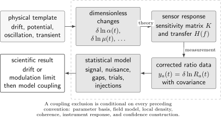
A variation search is a layered inference. A result at the right cannot be detached from the parameter convention, calculated sensitivities, instrument response, covariance, nuisance model, and statistical construction to its left.

Comparing Clocks and Spectra

Why a ratio is the observable

Any frequency measurement compares phase accumulation against another oscillator. Even an “absolute” optical frequency measured in hertz is a chain of comparisons to a realization of the SI second, presently based on the caesium-133 hyperfine transition.

For two simultaneously compared references,

$$y_{AB}(t) = \ln \left[ \frac{R_{AB}(t)}{R_{AB,0}} \right] \simeq \frac{R_{AB}(t)-R_{AB,0}}{R_{AB,0}}.$$

The logarithm makes small fractional changes additive and makes inversion simple:

$$y_{BA}(t) = -y_{AB}(t).$$

A sign error in the ratio order reverses a reported drift or coupling. The numerator, denominator, beat-note convention, comb mode numbers, and frequency offsets must therefore be frozen before analysis.

Three comparison geometries

Co-located optical ratio.
Two transitions are compared through one comb and often share an optical laboratory. Gravitational-potential differences and long links are small, while common environmental and comb errors can correlate the data.

Remote optical ratio.
Clock signals are transferred by stabilized fibre, free-space optical link, or satellite link. This enables networks and independent environments, but adds link phase, reference-plane, time-transfer, and relativistic corrections.

Optical-to-microwave absolute frequency.
An optical transition is compared with a caesium primary standard or time scale. This introduces sensitivity to $\mu$ and nuclear magnetic parameters that a purely electronic optical ratio may largely cancel. It also introduces dead time, flywheel oscillators, time-scale correlations, and the caesium systematic evaluation.

Molecular spectroscopy may compare a rovibrational transition with an atomic clock through a comb. Atom–cavity and molecule–cavity comparisons are also useful, but the cavity is a material sensor with its own frequency-dependent mechanical and thermal response, not a featureless reference.

The corrected time series

A raw ratio record can be represented as

$$y_i^{\mathrm{raw}} = s(t_i;\boldsymbol\vartheta) + \sum_a c_a z_a(t_i) + b_{r(i)} + n_i.$$

Here:

• $s(t;\boldsymbol\vartheta)$ is the proposed physical signal;
• $z_a(t)$ are monitored environmental or operational regressors;
• $c_a$ are nuisance couplings;
• $b_{r(i)}$ is a run-, configuration-, or reference-plane offset; and
• $\mathbf n$ has covariance $C$ that need not be diagonal or white.

The corrected record is not obtained by subtracting every correlated monitor. A regressor should be included because a physical or diagnostic model supports it, with uncertainty in its calibration propagated. Adding regressors after inspecting a candidate peak can absorb real signals or tune away noise.

Common references and closure

Suppose three simultaneous log ratios satisfy

$$y_{AB}+y_{BC}+y_{CA}=0.$$

The closure residual

$$\Delta_{\mathrm{cl}} = y_{AB}+y_{BC}+y_{CA}$$

tests consistency of counters, comb transfer, ratio signs, and reference planes. Its uncertainty includes covariance because the three ratios share clocks and transfer oscillators.

Closure does not test a common-mode variation to which all three transitions have identical sensitivity. It tests the comparison network.

Sampling and averaging are part of the detector

A reported point is usually an average over a gate of duration $T_g$:

$$\bar y(t) = \frac{1}{T_g} \int_{t-T_g/2}^{t+T_g/2} y(t')\,dt'.$$

For a sinusoidal input, rectangular averaging gives amplitude response

$$H_{\mathrm{gate}}(f) = \frac{ \sin(\pi fT_g) }{ \pi fT_g }.$$

Interrogation, servo, dead time, counter filtering, link processing, and subsequent binning add further transfer factors. A null result above the effective bandwidth does not constrain the unattenuated physical amplitude.

Sensitivity Coefficients

Definition

For transition $i$ and dimensionless parameter $X$,

$$K_{X,i} = \frac{\partial\ln\nu_i}{\partial\ln X}.$$

For a ratio,

$$\Delta K_X^{AB} = K_{X,A}-K_{X,B}.$$

Then

$$\delta\ln R_{AB} = \Delta K_\alpha^{AB} \frac{\delta\alpha}{\alpha} + \Delta K_\mu^{AB} \frac{\delta\mu}{\mu} + \Delta K_q^{AB} \frac{\delta X_q}{X_q} + \cdots.$$

The common dimensional frequency scale cancels. What remains is the differential dependence of the two physical systems.

Atomic electronic transitions

An electronic transition can be written schematically as

$$\nu_i = cR_\infty F_i(\alpha),$$

so

$$K_{\alpha,i} = \frac{\alpha}{F_i} \frac{\partial F_i}{\partial\alpha}$$

after the common $cR_\infty$ scale is factored out. Relativistic shifts grow roughly with $(Z\alpha)^2$, but level crossings and cancellations can produce much larger or sign-changing fractional sensitivities.

For two ordinary optical transitions, direct $\mu$ sensitivity is usually small because the leading electronic mass scale cancels. Isotope shifts, nuclear size, recoil, and hyperfine admixture can reintroduce nuclear-mass dependence.

Hyperfine transitions

A ground-state hyperfine frequency has the schematic scaling

$$\nu_{\mathrm{hfs}} \propto cR_\infty \alpha^2 F_{\mathrm{rel}}(\alpha) \frac{m_e}{m_p} g_I F_{\mathrm{nuc}},$$

where $g_I$ is a nuclear magnetic factor and $F_{\mathrm{nuc}}$ represents finite-size and nuclear-structure corrections. With $\mu=m_p/m_e$,

$$\delta\ln\nu_{\mathrm{hfs}} = \left( 2+K_{\mathrm{rel}} \right) \delta\ln\alpha - \delta\ln\mu + \delta\ln g_I + \delta\ln F_{\mathrm{nuc}} + \delta\ln(cR_\infty).$$

An optical-to-caesium comparison therefore does not constrain $\mu$ alone without assumptions or calculations for nuclear magnetic dependence. Calling it a “model-free proton-mass test” overstates the inference.

Molecular transitions

In a simple Born–Oppenheimer scaling picture,

$$\begin{aligned} \nu_{\mathrm{rot}} &\propto \mu^{-1}, \\ \nu_{\mathrm{vib}} &\propto \mu^{-1/2}, \\ \nu_{\mathrm{el}} &\propto \mu^0, \end{aligned}$$

where $\mu=m_p/m_e$ and the proportionalities refer to frequencies in a common electronic atomic scale. Hence the representative sensitivities are

$$K_{\mu,\mathrm{rot}} \simeq -1, \qquad K_{\mu,\mathrm{vib}} \simeq -\frac12.$$

Inversion, tunnelling, spin–orbit, and near-degenerate transitions can have enhanced coefficients. Enhancement often comes from cancellation between larger energy contributions, so theory uncertainty and field sensitivity must be assessed at the enhanced fractional level.

Sensitivities are calculated quantities

A reliable $K$ value should state:

• the definition and sign of every varied parameter;
• which other parameters were held fixed;
• the atomic, molecular, or nuclear Hamiltonian used;
• whether the derivative was analytic or obtained by finite differences;
• numerical convergence and many-body uncertainty;
• nuclear-size, polarizability, and magnetic-structure assumptions; and
• correlations among coefficients for related transitions.

At present clock precision, treating $K$ as an exact integer can be unjustified, especially for molecular enhancement or nuclear transitions.

Multiparameter identifiability

With $M$ measured ratios and $P$ varying parameters,

$$\mathbf y(t) = K\,\mathbf x(t) + \mathbf n(t),$$

where

$$K_{aX} = \Delta K_X^{(a)}.$$

If $\operatorname{rank}K<P$, the data constrain only combinations of parameters. Even at full rank, nearly parallel sensitivity rows make the inverse problem ill-conditioned.

For covariance $C$, the local information matrix is

$$\mathcal I = K^{\mathsf T}C^{-1}K.$$

Its small eigenvalues identify weakly measured combinations. Adding a transition is valuable when its sensitivity vector points in a new direction after its actual noise and covariance are included, not merely because its individual clock uncertainty is small.

One-coupling-at-a-time limits

Many exclusion plots set all but one coupling to zero. If

$$y = K_\alpha x_\alpha + K_\mu x_\mu,$$

then an alpha-only interpretation uses

$$x_\alpha = \frac{y}{K_\alpha} \quad \text{under the assumption} \quad x_\mu=0.$$

That result is useful, but it is not the marginalized bound in a two-parameter model. Papers and plots should label one-coupling-at-a-time, profiled, marginalized, and model-correlated limits distinctly.

Signal Models

Linear drift

The simplest phenomenological model is

$$x_X(t) = x_{X,0} + \dot x_X(t-t_0).$$

For one ratio,

$$y(t) = b + D(t-t_0) + n(t),$$

with

$$D = \sum_X \Delta K_X\dot x_X.$$

Choosing $t_0$ near the weighted mean observation time reduces covariance between intercept and slope. It does not change the slope.

A linear fit is meaningful only over its stated interval. Instrument upgrades, relocks, transport, reference changes, software changes, and step-like systematic shifts can imitate or obscure a slope. A mature analysis compares:

• one global intercept against documented run-dependent offsets;
• white-noise against colored-noise covariance;
• a slope fitted before and after each major intervention;
• raw and correction-applied records;
• leave-one-run-out and leave-one-season-out results; and
• fixed analysis choices against blinded or preregistered choices.

The notation

$$\frac{\dot\alpha}{\alpha}$$

means the fitted local fractional drift rate under this model. It does not claim that the same linear law held over geological or cosmological time.

Gravitational-potential modulation

A phenomenological local-position-invariance test can write

$$\delta\ln X = k_X \frac{\Delta U}{c^2},$$

where $U$ is a declared gravitational potential per unit mass and $k_X$ is a dimensionless coupling. A clock ratio then has

$$\delta\ln R_{AB} = \left( \sum_X \Delta K_X^{AB}k_X \right) \frac{\Delta U}{c^2}.$$

Earth’s orbital eccentricity modulates the solar potential. To first order,

$$\frac{\Delta U_\odot(t)}{c^2} \simeq \frac{ e_{\oplus}GM_\odot }{ a_{\oplus}c^2 } \cos \left[ \Omega_\oplus(t-t_p) \right].$$

The sinusoidal amplitude is about

$$1.65\times10^{-10},$$

while the perihelion-to-aphelion difference is twice that value. A report must say whether it quotes amplitude or peak-to-peak change.

General relativity predicts a universal gravitational redshift. A co-located ratio is sensitive to species-dependent anomalous response, not to the common universal term. Remote clocks additionally require the ordinary relativistic potential and velocity corrections before a nonuniversal residual is interpreted.

An annual fit is vulnerable to annual laboratory systematics: temperature, humidity, magnetic fields, blackbody environments, grounding, air-conditioning operation, link availability, and maintenance. The solar phase is fixed by the ephemeris. Fitting an arbitrary annual phase after looking at the data changes the hypothesis and its degrees of freedom.

Deterministic oscillation

At fixed angular frequency $\omega$,

$$y(t) = a_\omega\cos\omega t + b_\omega\sin\omega t + \mathbf z(t)^{\mathsf T}\boldsymbol\gamma + n(t).$$

The quadrature amplitude and phase are

$$A_\omega = \sqrt{a_\omega^2+b_\omega^2}, \qquad \varphi_\omega = \operatorname{atan2}(-b_\omega,a_\omega),$$

for the convention

$$A_\omega\cos(\omega t+\varphi_\omega).$$

The sign in the phase definition changes if the sine convention changes. Amplitude is nonnegative, so its null distribution is not a centred Gaussian even when the fitted quadratures are Gaussian.

Stochastic narrowband signal

An ultralight field drawn from a virialized halo need not preserve one phase over an arbitrarily long dataset. It is more accurately a narrowband stochastic process with finite coherence time. If the observation time is short compared with that time, a coherent sinusoid is a good approximation. If it is much longer, the likelihood should account for phase decorrelation and the expected line shape.

The deterministic and stochastic analyses answer different questions. Using a single coherent sinusoid across many coherence times can lose sensitivity or give incorrect coverage.

Transient signal

A transient model may predict a localized pulse, step, dispersive feature, or a sequence of arrival times across a network:

$$y_a(t) = A_a g \left[ \frac{ t-t_0-\tau_a(\widehat{\mathbf v}) }{ \tau } \right] + n_a(t).$$

Here $a$ labels the sensor, $g$ is a declared waveform, $\tau$ is a duration, and $\tau_a$ is the geometric arrival delay. A credible network candidate must exhibit:

• the predicted relative signs and amplitudes from the sensitivity coefficients;
• arrival times compatible with one propagation direction and speed;
• no corresponding link, time-transfer, power, magnetic, or environmental disturbance;
• calibrated response at the candidate duration; and
• a global significance that includes the event-time, duration, and direction scan.

A simultaneous clock glitch is not automatically a dark-matter event, especially when the clocks share a time scale, transfer oscillator, comb, software pipeline, or environmental disturbance.

Fine-Structure Constant Variation

Differential relativistic sensitivity

The best alpha searches pair transitions with large

$$\left| \Delta K_\alpha \right|.$$

Relativistic level shifts in heavy atoms and ions provide leverage. Transitions near an accidental cancellation or level crossing can enhance fractional sensitivity further, but may bring difficult polarizability, quadrupole, magnetic, or many-body corrections.

The electric-octupole E3 and electric-quadrupole E2 transitions in $^{171}\mathrm{Yb}^+$ are a particularly useful pair. Their alpha sensitivities differ by approximately

$$\Delta K_\alpha^{\mathrm{E3/E2}} \simeq -6.95.$$

Both transitions can be interrogated in the same trapped ion. This removes species transport and greatly reduces some link uncertainties, while interleaved operation still leaves time-offset sampling and transition-specific systematic effects.

Converting ratio drift

For an alpha-only model,

$$\frac{d}{dt} \ln \left( \frac{\nu_{\mathrm{E3}}}{\nu_{\mathrm{E2}}} \right) = \Delta K_\alpha^{\mathrm{E3/E2}} \frac{\dot\alpha}{\alpha}.$$

Thus

$$\frac{\dot\alpha}{\alpha} = \frac{ d\ln(\nu_{\mathrm{E3}}/\nu_{\mathrm{E2}})/dt }{ \Delta K_\alpha^{\mathrm{E3/E2}} }.$$

The negative $\Delta K_\alpha$ reverses the sign between ratio drift and alpha drift.

Using long-term E3/E2 data through 2022, Filzinger and collaborators reported

$$\frac{\dot\alpha}{\alpha} = 1.8(2.5)\times10^{-19}\ {\rm yr^{-1}},$$

consistent with zero. In the solar-potential model they found

$$\frac{c^2}{\alpha} \frac{d\alpha}{dU_\odot} = -2.4(3.0)\times10^{-9},$$

also consistent with zero. As of this page’s review date, these are among the strongest direct laboratory clock constraints on the specified linear drift and solar-potential templates.

The parentheses are one-standard-deviation fit uncertainties, not a detection interval. A two-sided upper limit requires a declared confidence construction rather than simply replacing the central value by zero.

Earlier independent comparisons

The $^{27}\mathrm{Al}^+/^{199}\mathrm{Hg}^+$ optical ratio established the modern direct-clock strategy. Repeated comparisons gave

$$\frac{\dot\alpha}{\alpha} = \left( -1.6\pm2.3 \right) \times10^{-17}\ {\rm yr^{-1}}$$

in 2008. Later $^{171}\mathrm{Yb}^+$, strontium, dysprosium, and atom–cavity measurements extended the time span, sensitivity basis, and frequency reach.

Older results remain valuable because independent atoms, laboratories, systematics, and sampling windows can reject an apparatus-specific periodicity that a more precise single dataset cannot diagnose alone.

Alpha-search systematics

Important false channels include:

• transition-specific blackbody, dc Stark, quadrupole, Zeeman, and probe shifts;
• clock-state-dependent servo or line-pulling effects;
• comb transfer and acousto-optic frequency-offset signs;
• time-dependent ion motion, trap fields, or lattice conditions;
• reference-cavity changes in atom–cavity comparisons;
• annual environmental cycles in solar-potential fits;
• maintenance steps mistaken for drift; and
• aliases of diurnal or operational cycles into a sparse spectral window.

Large $\Delta K_\alpha$ does not suppress these effects. It only converts a given ratio residual into a smaller inferred $\delta\alpha/\alpha$.

Proton-to-Electron Mass-Ratio Variation

Optical and microwave complementarity

With

$$\mu=\frac{m_p}{m_e},$$

purely electronic optical ratios have weak leading sensitivity to $\mu$. Comparing an optical transition with a hyperfine standard introduces the factor $m_e/m_p=\mu^{-1}$ and therefore stronger mass-ratio leverage.

For optical reference $o$ and hyperfine reference $h$,

$$\delta\ln \left( \frac{\nu_o}{\nu_h} \right) = \Delta K_\alpha\,\delta\ln\alpha + \Delta K_\mu\,\delta\ln\mu + \Delta K_g\,\delta\ln g_I + \cdots.$$

Multiple ratios are required to separate alpha, mass-ratio, and nuclear magnetic terms without one-at-a-time assumptions.

Combining the $^{171}\mathrm{Yb}^+$ E3/E2 optical ratio with E3-to-caesium absolute-frequency data, Lange and collaborators obtained

$$\frac{\dot\mu}{\mu} = -8(36)\times10^{-18}\ {\rm yr^{-1}}$$

and a solar-potential coupling

$$\frac{c^2}{\mu} \frac{d\mu}{dU_\odot} = 7(45)\times10^{-8}$$

in 2021. Both results are consistent with zero. They rely on the declared $\mu=m_p/m_e$ convention and on the sensitivity model for the caesium hyperfine reference.

Molecular leverage

Rotational, vibrational, inversion, and tunnelling transitions can probe $\mu$ with a different structure-theory basis. Useful strategies include:

• comparing vibrational overtones over several years;
• comparing rotational and vibrational lines in one molecule;
• comparing molecular and atomic references through a comb;
• using near-degenerate transitions with enhanced differential sensitivity; and
• combining isotopologues to change nuclear-mass dependence.

The tradeoff is that a molecule may have larger Stark, Zeeman, blackbody, collision, motion, and line-shape sensitivities than a clock transition. Enhanced $K_\mu$ is useful only after the long-term systematic reproducibility is demonstrated.

What does a changing proton mass mean?

Most of the proton mass arises from QCD dynamics, not the sum of bare valence-quark masses. A microscopic scalar model may change

$$\Lambda_{\mathrm{QCD}}, \qquad m_u,\ m_d,\ m_s, \qquad m_e, \qquad \alpha$$

with different couplings. The observable

$$\delta\ln\mu = \delta\ln m_p - \delta\ln m_e$$

is model-independent, but translating it into quark, gluon, or electron-sector couplings requires hadronic and nuclear response coefficients. The shorthand “proton-mass coupling” should not conceal that model layer.

Ultralight Scalar Dark Matter Overview

Classical-field regime

A sufficiently occupied ultralight bosonic mode can be treated as a classical field. In natural units $\hbar=c=1$, a simple local model is

$$\phi(t,\mathbf x) \simeq \phi_0 \cos \left( m_\phi t-\mathbf k_\phi\mathbin{\cdot}\mathbf x+\theta \right),$$

with

$$\phi_0 \simeq \frac{\sqrt{2\rho_\phi}}{m_\phi}.$$

Restoring ordinary frequency units,

$$f_\phi = \frac{m_\phi c^2}{h}.$$

The field density $\rho_\phi$ may be the full adopted local dark-matter density or only a fraction of it. Every coupling exclusion must state that choice.

For a virial speed

$$v\sim10^{-3}c,$$

the fractional linewidth is of order

$$\frac{\Delta f}{f_\phi} \sim \frac{v^2}{c^2} \sim 10^{-6}.$$

Equivalently, the coherence quality factor is roughly

$$Q_\phi \sim \frac{f_\phi}{\Delta f} \sim 10^6.$$

Order-unity factors depend on the halo velocity distribution and coherence definition.

Coupling to effective constants

One common linear-coupling convention writes

$$\begin{aligned} \delta\ln\alpha &= d_e\kappa\phi, \\ \delta\ln\mu &= d_\mu\kappa\phi, \end{aligned}$$

where $\kappa$ is an inverse-energy normalization, often built from Newton’s constant. Then a ratio has oscillation amplitude

$$A_{AB} = \left| \Delta K_\alpha d_e + \Delta K_\mu d_\mu + \cdots \right| \kappa \frac{\sqrt{2\rho_\phi}}{m_\phi}.$$

This equation makes the conditional structure visible:

• the same ratio-amplitude limit gives a coupling limit proportional to $m_\phi$ under fixed density;
• different parameter bases rotate the coupling combination;
• the inferred limit weakens if the field is only a fraction of local dark matter;
• coherence and detector response determine the applicable likelihood; and
• one-coupling-at-a-time curves set the other $d_X$ to zero.

Numerical values of $d_e$ from different papers must not be compared until their $\kappa$, field normalization, density, and confidence convention match.

Linear and quadratic portals

For a linear coupling, the dominant variation is at $f_\phi$. For a quadratic coupling,

$$\delta\ln X = d_X^{(2)} \left( \kappa\phi \right)^2,$$

and

$$\phi^2(t) = \frac{\phi_0^2}{2} \left[ 1+\cos(2\omega_\phi t+2\theta) \right].$$

The observable contains a constant offset and an oscillation at $2f_\phi$. A search at only $f_\phi$ does not constrain this model in the same way.

What clock searches have established

Clock, atom–cavity, atomic-spectroscopy, and molecular-spectroscopy records have searched broad but finite mass ranges. For example, the 2023 $^{171}\mathrm{Yb}^+$ E3/E2 and E3/strontium analysis improved photon-coupling limits over much of approximately

$$10^{-24} \lesssim \frac{m_\phi}{\mathrm{eV}/c^2} \lesssim 10^{-17}$$

under its scalar-field and halo assumptions. Optical-to-microwave clock records add electron, quark, and gluon sensitivity; radio-frequency atomic and molecular spectroscopy extends to higher oscillation frequencies.

These experiments reported no significant dark-matter signal. Their exclusion curves are complementary, not interchangeable: each covers a particular mass band, coupling basis, field model, duty cycle, and sensor response.

Transient field structures

Some models allow macroscopic domain walls or other field structures that produce transient changes rather than a stationary narrowband signal. Atomic-clock networks, including archival satellite-clock networks, have searched for propagating correlated disturbances and found no signal at their stated sensitivities.

The existence, abundance, encounter rate, profile, and coupling of such structures are additional assumptions. A transient exclusion should state whether it is conditional on those objects making all dark matter and how the non-observation is converted into an encounter-rate or coupling bound.

Statistical Analysis

Generalized least squares

For a fixed signal template, collect the observations into

$$\mathbf y = X\boldsymbol\beta + \mathbf n, \qquad \operatorname{cov}(\mathbf n)=C.$$

The design matrix may contain an intercept, drift, sine and cosine quadratures, environmental regressors, and run offsets. The generalized-least-squares estimator is

$$\widehat{\boldsymbol\beta} = \left( X^{\mathsf T}C^{-1}X \right)^{-1} X^{\mathsf T}C^{-1}\mathbf y,$$

with covariance

$$V_\beta = \left( X^{\mathsf T}C^{-1}X \right)^{-1}$$

when $C$ is known and the linear-Gaussian model is adequate.

Estimating $C$ from the same residuals adds uncertainty. Red noise, random-walk frequency noise, servo transients, and run-correlated systematics should be tested rather than hidden by rescaling all point errors to make reduced $\chi^2$ equal to one.

Irregular sampling and the spectral window

For sample times $t_i$, the window

$$W(\omega) = \sum_i w_i e^{-i\omega t_i}$$

determines aliases and correlations among scanned frequencies. Daily operation, weekdays, seasonal uptime, and long gaps can move power from one frequency to another.

A Lomb–Scargle periodogram or equivalent likelihood scan handles irregular times more appropriately than a naive discrete Fourier transform, but it does not by itself solve:

• colored or heteroscedastic noise;
• time averaging and servo attenuation;
• run-dependent offsets;
• shared systematics among ratios;
• frequency-dependent theory response; or
• the global trials factor.

The safest procedure is to define a generative model, simulate or inject signals through the actual timestamps and processing, and verify recovery.

Local and global significance

At one prespecified frequency, a test statistic has a local significance. Scanning $N_{\mathrm{eff}}$ effectively independent frequencies raises the chance of a noise maximum. In the simple independent approximation,

$$p_{\mathrm{global}} = 1- \left( 1-p_{\mathrm{local}} \right)^{N_{\mathrm{eff}}} \simeq N_{\mathrm{eff}}p_{\mathrm{local}}$$

for small $p_{\mathrm{local}}$. Real frequency bins are correlated, so $N_{\mathrm{eff}}$ is best calibrated with noise simulations or an appropriate extreme-value model.

Event-time, duration, waveform, direction, coupling, and subset scans also create trials. Reporting only the most impressive local peak is incomplete.

Upper limits and coverage

A null search should declare:

• frequentist confidence level or Bayesian credible level;
• the likelihood and prior, if any;
• whether nuisance parameters were profiled or marginalized;
• whether the limit is pointwise or simultaneous over a band;
• treatment of the nonnegative amplitude boundary;
• power constraints or sensitivity bands;
• calibration of coverage with synthetic data; and
• conversion from ratio amplitude to parameter or coupling space.

Expected sensitivity bands distinguish an unusually strong limit caused by a downward noise fluctuation from a robust experimental improvement.

Signal injections

End-to-end injections should test:

1. timestamp and time-scale conversion;
2. phase and ratio-sign conventions;
3. gate, servo, and link transfer functions;
4. gaps and data-quality cuts;
5. covariance estimation;
6. nuisance-regressor absorption;
7. frequency and event-parameter recovery;
8. local and global significance calibration; and
9. final coupling conversion.

Software-unit tests are necessary but cannot replace injections through the actual analysis chain.

Network covariance

For sensors $a$ and $b$,

$$C_{ab}(t,t') = \left\langle n_a(t)n_b(t') \right\rangle.$$

Off-diagonal covariance can arise from:

• one shared reference clock or time scale;
• common combs, links, or flywheel oscillators;
• environmental fields over a site;
• common theory coefficients;
• shared correction models; and
• global data-selection or time-transfer processing.

A network gains discovery power through independent sensitivity, geographical timing, and redundant closure. Counting correlated channels as independent produces overconfident limits.

Experimental Strategy

Choosing references

A strong campaign balances:

• large and complementary sensitivity coefficients;
• demonstrated long-term systematic reproducibility;
• high duty cycle and timestamp integrity;
• independent apparatus and environmental conditions;
• transfer links with calibrated phase response;
• enough baseline for the target low frequency;
• enough sampling bandwidth for the target high frequency; and
• theory coefficients accurate relative to the desired parameter limit.

The clock with the smallest headline systematic uncertainty is not always the best variation sensor. A less accurate reference with a much larger differential sensitivity or duty cycle can carry more information for a specific signal.

Reversal and modulation channels

Useful controls include:

• alternating transition, Zeeman, hyperfine, or molecular state;
• reversing magnetic field, polarization, propagation direction, or molecular orientation;
• changing trap depth, probe power, and blackbody environment over a deliberate lever arm;
• comparing independent combs or links;
• reprocessing with documented correction variants; and
• hiding the final ratio, drift, or injected offset until analysis choices are frozen.

A new-field signal follows the sensitivity-coefficient pattern. A systematic often follows an operational coordinate. Deliberate modulation helps distinguish them.

Environmental regressors

Temperature, magnetic field, electric field, pressure, humidity, laser power, trap parameters, cavity diagnostics, oscillator state, and link health should be recorded continuously. Their sensors need calibration, timestamps, bandwidth, and uncertainty commensurate with the searched signal.

Regressors can be collinear with a target template. For example, an annual temperature term may be nearly degenerate with a solar-potential modulation. The fit must report this covariance rather than claim that including temperature automatically solved the problem.

Common Mistakes

Asking whether a dimensional number changed without defining the reference.
The operational claim must be expressed through a dimensionless ratio or a fully specified unit realization.

Using one clock alone.
A clock output is already a comparison between an atom and an oscillator. Interpreting its drift requires another physical reference with different sensitivity.

Forgetting the mass-ratio convention.
$m_p/m_e$ and $m_e/m_p$ give opposite $K_\mu$ and drift signs.

Treating sensitivity coefficients as exact labels.
They come from structure calculations and may share theory uncertainty.

Converting one ratio into several independently varied constants.
One scalar time series constrains one combination unless additional independent sensitivities or priors are supplied.

Calling an annual residual a gravitational effect.
Seasonal laboratory variables and data availability can have the same period. The solar phase, environmental model, and alternative hypotheses must be tested.

Ignoring the detector transfer function.
Gate averaging, interrogation, servos, counters, and links attenuate or phase-shift fast signals.

Reading the largest periodogram peak as a discovery.
The global trials factor, colored noise, aliases, and analysis choices belong in the significance.

Equating an oscillation limit with a model-independent dark-matter limit.
The coupling curve assumes a field normalization, density fraction, coherence, halo distribution, and coupling basis.

Treating network channels as independent.
Shared references, links, corrections, and time scales create cross-covariance.

Fitting away inconvenient structure.
Post hoc run offsets or environmental regressors can absorb either a systematic or a real signal. Their use needs a predeclared or physically validated rationale.

Reporting Checklist

Layer	What to report
Observable	Ratio order, transitions, isotopes, states, and reference planes
Timing	Time scale, timestamp uncertainty, gates, duty cycle, gaps, and baseline
Sensitivity	Parameter definitions, $K$ values, theory method, uncertainty, and covariance
Corrections	Applied values, signs, environmental monitors, and run changes
Response	Interrogation, servo, counter, link, and averaging transfer functions
Noise	Point covariance, colored-noise model, cross-channel covariance, and diagnostics
Template	Drift interval, ephemeris phase, oscillation coherence, or transient waveform
Statistics	Likelihood, nuisance treatment, scan range, trials, injections, and coverage
Interpretation	One-at-a-time or joint parameters, field normalization, density, and halo model
Result	Primary ratio residuals, phenomenological limit, then conditional coupling limit

Publishing the corrected ratio series and metadata is especially valuable. Future theory or halo assumptions can then be applied without reverse-engineering an exclusion curve from a raster plot.

Exercises

Exercise 1: Ratio order and alpha drift

A ratio $R=\nu_A/\nu_B$ has

$$\Delta K_\alpha=K_{\alpha,A}-K_{\alpha,B}=-4.$$

Its measured logarithmic drift is

$$\frac{d\ln R}{dt} = 8.0\times10^{-18}\ {\rm yr^{-1}}.$$

Assuming only $\alpha$ varies, find $\dot\alpha/\alpha$. What value would be inferred if an analyst accidentally used $R^{-1}$ but kept $\Delta K_\alpha=-4$?

Solution

The correct inference is

$$\frac{\dot\alpha}{\alpha} = \frac{1}{\Delta K_\alpha} \frac{d\ln R}{dt} = -2.0\times10^{-18}\ {\rm yr^{-1}}.$$

For the inverse ratio,

$$\frac{d\ln R^{-1}}{dt} = -8.0\times10^{-18}\ {\rm yr^{-1}},$$

and its correct sensitivity is $+4$. Keeping the old sensitivity by mistake would give

$$+2.0\times10^{-18}\ {\rm yr^{-1}},$$

the wrong sign. Ratio and sensitivity conventions must be inverted together.

Exercise 2: Two ratios and two varying parameters

Two measured ratio changes obey

$$\begin{pmatrix} y_1\\ y_2 \end{pmatrix} = \begin{pmatrix} 2 & -1\\ 5 & 1 \end{pmatrix} \begin{pmatrix} x_\alpha\\ x_\mu \end{pmatrix}.$$

For $y_1=3\times10^{-17}$ and $y_2=4\times10^{-17}$, solve for $x_\alpha$ and $x_\mu$.

Solution

The equations are

$$2x_\alpha-x_\mu=3\times10^{-17},$$

and

$$5x_\alpha+x_\mu=4\times10^{-17}.$$

Adding gives

$$7x_\alpha=7\times10^{-17},$$

so

$$x_\alpha=1.0\times10^{-17}.$$

Substitution gives

$$x_\mu = 2x_\alpha-3\times10^{-17} = -1.0\times10^{-17}.$$

One ratio alone would constrain only a line in $(x_\alpha,x_\mu)$ space. The nonparallel sensitivity rows make the two-parameter solution identifiable.

Exercise 3: Ytterbium-ion ratio conversion

Use

$$\Delta K_\alpha^{\mathrm{E3/E2}}=-6.95$$

and

$$\frac{\dot\alpha}{\alpha} = 1.8\times10^{-19}\ {\rm yr^{-1}}$$

to find the corresponding best-fit drift of $\ln(\nu_{\mathrm{E3}}/\nu_{\mathrm{E2}})$. Repeat for the $2.5\times10^{-19}\ {\rm yr^{-1}}$ standard uncertainty.

Solution

The ratio drift is

$$\begin{aligned} D_R &= \Delta K_\alpha \frac{\dot\alpha}{\alpha} \\ &= -6.95 \left( 1.8\times10^{-19} \right) \\ &= -1.25\times10^{-18}\ {\rm yr^{-1}}. \end{aligned}$$

The standard uncertainty is

$$u(D_R) = 6.95 \left( 2.5\times10^{-19} \right) = 1.74\times10^{-18}\ {\rm yr^{-1}}.$$

Thus the underlying fitted ratio drift is also consistent with zero.

Exercise 4: Solar-potential modulation

Suppose an alpha-sensitive ratio has $\Delta K_\alpha=-7$ and the coupling model has $k_\alpha=3\times10^{-9}$. Estimate the annual ratio-modulation amplitude using

$$\left| \frac{\Delta U_\odot}{c^2} \right|_{\mathrm{amp}} = 1.65\times10^{-10}.$$

Solution

The ratio amplitude is

$$\begin{aligned} A_R &= \left| \Delta K_\alpha k_\alpha \right| \left| \frac{\Delta U_\odot}{c^2} \right|_{\mathrm{amp}} \\ &= 7 \left( 3\times10^{-9} \right) \left( 1.65\times10^{-10} \right) \\ &= 3.47\times10^{-18}. \end{aligned}$$

The sign and phase carry additional information: $\Delta K_\alpha k_\alpha<0$ specifies whether the ratio is largest near perihelion or aphelion under the adopted potential sign. Reporting only the absolute amplitude discards that check.

Exercise 5: Gate attenuation

A clock ratio is averaged in nonoverlapping $T_g=1000\ {\rm s}$ gates. Find the magnitude of the rectangular-gate response for signals at

$$f_1=10^{-4}\ {\rm Hz} \quad\text{and}\quad f_2=10^{-3}\ {\rm Hz}.$$

Solution

The response is

$$H(f) = \frac{\sin(\pi fT_g)}{\pi fT_g}.$$

For $f_1$,

$$\pi f_1T_g = 0.1\pi,$$

so

$$|H(f_1)| = \frac{\sin(0.1\pi)}{0.1\pi} \simeq 0.984.$$

For $f_2$,

$$\pi f_2T_g=\pi,$$

and therefore

$$H(f_2)=0.$$

The second signal averages to zero for ideal rectangular gates. An exclusion that ignores this transfer zero would be invalid.

Exercise 6: Dark-matter mass, frequency, and coherence

For

$$m_\phi=10^{-18}\ {\rm eV}/c^2,$$

use

$$\frac{1\ {\rm eV}}{h} = 2.418\times10^{14}\ {\rm Hz}$$

to estimate $f_\phi$. If $Q_\phi=10^6$, estimate the coherence time

$$\tau_c \sim \frac{Q_\phi}{f_\phi}.$$

Solution

The oscillation frequency is

$$f_\phi = 10^{-18} \left( 2.418\times10^{14} \right) = 2.418\times10^{-4}\ {\rm Hz}.$$

The period is about

$$T_\phi = \frac{1}{f_\phi} \simeq 4.14\times10^3\ {\rm s},$$

or $69$ minutes. The coherence time estimate is

$$\tau_c \sim \frac{10^6}{2.418\times10^{-4}} \simeq 4.14\times10^9\ {\rm s},$$

about $131$ years. Order-unity factors depend on whether coherence is defined with angular or cyclic frequency and on the halo line shape. For a campaign much shorter than this, a coherent-sinusoid approximation is reasonable.

Exercise 7: Look-elsewhere correction

A frequency scan has a smallest local tail probability

$$p_{\mathrm{local}}=2\times10^{-5}$$

among $N_{\mathrm{eff}}=1000$ independent frequencies. Estimate the global tail probability.

Solution

Use

$$p_{\mathrm{global}} = 1- \left( 1-p_{\mathrm{local}} \right)^{N_{\mathrm{eff}}}.$$

Numerically,

$$p_{\mathrm{global}} \simeq 1-e^{-0.02} \simeq 0.0198.$$

The small-$p$ approximation gives

$$N_{\mathrm{eff}}p_{\mathrm{local}} = 0.020,$$

which agrees well. A locally striking peak is not globally compelling after the scan.

Exercise 8: Quadratic coupling

Let

$$\phi(t) = \phi_0\cos\omega_\phi t$$

and

$$\delta\ln X = d_X^{(2)} \left( \kappa\phi \right)^2.$$

Find the constant and oscillating parts of $\delta\ln X$. At what frequency should a search look?

Solution

Using

$$\cos^2\omega_\phi t = \frac12 \left( 1+\cos2\omega_\phi t \right),$$

we obtain

$$\delta\ln X = \frac{ d_X^{(2)}\kappa^2\phi_0^2 }{2} + \frac{ d_X^{(2)}\kappa^2\phi_0^2 }{2} \cos2\omega_\phi t.$$

The first term is a constant offset and the second oscillates at

$$2f_\phi.$$

A clock-ratio search is generally insensitive to an unknown static offset because it is absorbed into the fitted baseline. Its direct signature is therefore the $2f_\phi$ modulation.

Further Connections

• Fundamental Constants develops the fixed-epoch observational equations and CODATA adjustment that underlie the parameter definitions.
• Optical Clocks develops ion and lattice architectures, ratio comparison, systematic shifts, and relativistic reference planes.
• Atomic Clocks develops interrogation, local oscillators, servos, dead time, and the Dick effect.
• Frequency Standards develops Allan statistics, traceability, time scales, flywheels, and comparison links.
• Precision Spectroscopy develops line-centre inference and the anomaly-control workflow.
• Atom-Interferometric Sensors develops phase response, reversals, transfer functions, and network-ready inertial sensing.
• Cold Molecules develops molecular preparation, trapping, state control, and systematic reversals relevant to enhanced $\mu$ sensitivity.
• Fundamental Symmetry Frontiers distinguishes oscillating cosmic-field searches from static fifth-force, EDM, parity-violation, and isotope-shift programs.
• Fisher Information gives the canonical multiparameter information geometry.

References

Reviews and clock principles

1. J.-P. Uzan, Varying constants, gravitation and cosmology, Living Rev. Relativ. 14, 2 (2011).
2. M. S. Safronova, D. Budker, D. DeMille, D. F. Jackson Kimball, A. Derevianko, and C. W. Clark, Search for new physics with atoms and molecules, Rev. Mod. Phys. 90, 025008 (2018).
3. A. D. Ludlow, M. M. Boyd, J. Ye, E. Peik, and P. O. Schmidt, Optical atomic clocks, Rev. Mod. Phys. 87, 637–701 (2015).
4. V. V. Flambaum and M. G. Kozlov, Enhanced sensitivity to the time-variation of the fine-structure constant and $m_p/m_e$ in diatomic molecules, Phys. Rev. Lett. 99, 150801 (2007).

Drift and gravitational-potential tests

5. T. Rosenband, D. B. Hume, P. O. Schmidt, et al., Frequency ratio of $\mathrm{Al}^+$ and $\mathrm{Hg}^+$ single-ion optical clocks; metrology at the 17th decimal place, Science 319, 1808–1812 (2008).
6. R. M. Godun, P. B. R. Nisbet-Jones, J. M. Jones, et al., Frequency ratio of two optical clock transitions in $^{171}\mathrm{Yb}^+$ and constraints on the time variation of fundamental constants, Phys. Rev. Lett. 113, 210801 (2014).
7. N. Huntemann, B. Lipphardt, C. Tamm, V. Gerginov, S. Weyers, and E. Peik, Improved limit on a temporal variation of $m_p/m_e$ from comparisons of $\mathrm{Yb}^+$ and Cs atomic clocks, Phys. Rev. Lett. 113, 210802 (2014).
8. R. Lange, N. Huntemann, J. M. Rahm, et al., Improved limits for violations of local position invariance from atomic clock comparisons, Phys. Rev. Lett. 126, 011102 (2021).
9. M. Filzinger, S. Dörscher, R. Lange, et al., Improved limits on the coupling of ultralight bosonic dark matter to photons from optical atomic clock comparisons, Phys. Rev. Lett. 130, 253001 (2023).
10. N. Sherrill, A. O. Parsons, C. F. A. Baynham, et al., Analysis of atomic-clock data to constrain variations of fundamental constants, New J. Phys. 25, 093012 (2023).

Oscillating ultralight fields

11. K. Van Tilburg, N. Leefer, L. Bougas, and D. Budker, Search for ultralight scalar dark matter with atomic spectroscopy, Phys. Rev. Lett. 115, 011802 (2015).
12. A. Hees, J. Guéna, M. Abgrall, S. Bize, and P. Wolf, Searching for an oscillating massive scalar field as a dark matter candidate using atomic hyperfine frequency comparisons, Phys. Rev. Lett. 117, 061301 (2016).
13. D. Antypas, O. Tretiak, A. Garcon, R. Ozeri, G. Perez, and D. Budker, Scalar dark matter in the radio-frequency band: atomic-spectroscopy search results, Phys. Rev. Lett. 123, 141102 (2019).
14. C. J. Kennedy, E. Oelker, J. M. Robinson, et al., Precision metrology meets cosmology: improved constraints on ultralight dark matter from atom–cavity frequency comparisons, Phys. Rev. Lett. 125, 201302 (2020).
15. T. Kobayashi, A. Takamizawa, D. Akamatsu, et al., Search for ultralight dark matter from long-term frequency comparisons of optical and microwave atomic clocks, Phys. Rev. Lett. 129, 241301 (2022).
16. R. Oswald, A. Nevsky, V. Vogt, et al., Search for dark-matter-induced oscillations of fundamental constants using molecular spectroscopy, Phys. Rev. Lett. 129, 031302 (2022).
17. O. Tretiak, X. Zhang, N. L. Figueroa, et al., Improved bounds on ultralight scalar dark matter in the radio-frequency range, Phys. Rev. Lett. 129, 031301 (2022).
18. X. Zhang, A. Banerjee, M. Leyser, et al., Search for ultralight dark matter with spectroscopy of radio-frequency atomic transitions, Phys. Rev. Lett. 130, 251002 (2023).

Networks and transients

19. A. Derevianko and M. Pospelov, Hunting for topological dark matter with atomic clocks, Nat. Phys. 10, 933–936 (2014).
20. B. M. Roberts, G. Blewitt, C. Dailey, et al., Search for domain wall dark matter with atomic clocks on board global positioning system satellites, Nat. Commun. 8, 1195 (2017).
21. P. Wcisło, P. Ablewski, K. Beloy, et al., New bounds on dark matter coupling from a global network of optical atomic clocks, Sci. Adv. 4, eaau4869 (2018).
22. B. M. Roberts, P. Delva, A. Al-Masoudi, et al., Search for transient variations of the fine structure constant and dark matter using fiber-linked optical atomic clocks, New J. Phys. 22, 093010 (2020).
23. K. Beloy et al. (BACON Collaboration), Frequency ratio measurements at 18-digit accuracy using an optical clock network, Nature 591, 564–569 (2021).