Light–Matter Interaction

Light–matter interaction is the coupling of charged quantum systems to electromagnetic fields. The phrase covers several distinct models: a prescribed classical laser driving an atom, a molecule exchanging excitations with a quantized cavity mode, an excited state radiating into a continuum, and a detector conditioning a quantum state on the emitted record. They are connected, but they are not interchangeable.

The Quantum Optics chapter takes the next operational step: it treats selected field modes as systems whose states, transformations, correlations, and measurements are themselves the target.

A useful starting decomposition is

$$H = H_{\mathrm{matter}} + H_{\mathrm{field}} + H_{\mathrm{int}} + H_{\mathrm{environment}}.$$

The first question is not “which famous Hamiltonian applies?” It is:

Which matter, field, environmental, and detector degrees of freedom must remain dynamical for the observable and accuracy of interest?

Every practical light–matter model answers that question by approximation. The trustworthy route is to state the parent theory, identify each dimensionless small parameter, and verify that discarded degrees of freedom do not control the measured signal.

Canonical Scope

This page is the map of model choices. It owns the handoffs between:

1. microscopic electromagnetic coupling;
2. prescribed classical fields and quantized radiation;
3. dipole, multipole, and few-level reductions;
4. closed coherent dynamics and open dissipative dynamics;
5. spectroscopy, control, and measurement.

Detailed derivations live elsewhere:

• Minimal Coupling owns the AMO many-charge Hamiltonian, its $p\cdot A$ and $A^2$ terms, and classical versus quantized field bookkeeping. The geometric treatment owns the underlying gauge-covariance argument.
• Quantized Electromagnetic Modes owns the source-free Maxwell-mode reduction, oscillator quantization, zero-point field scale, continuum normalization, and mode-volume cautions.
• Gauge Choices in Light–Matter Physics owns the Coulomb, velocity, length, and multipolar representation dictionary and its truncation tests.
• Dipole Approximation owns the internal long-wavelength expansion, transition-dipole interpretation, center-of-mass phase distinction, and validity tests.
• Multipole Expansion owns the E1, M1, E2, and higher interaction hierarchy, field-gradient couplings, free-space rate scaling, and forbidden-line applications.
• Two-Level Atom owns the controlled reduction from a multilevel spectrum to a driven two-state Hamiltonian, including frame and detuning conventions.
• Dipole Transitions owns the symmetry and polarization selection rules.
• Transition Rates in Light–Matter Interaction owns the $N$ versus $N+1$ rate dictionary and the free-space spontaneous-emission rate.
• Spontaneous Emission owns the vacuum-continuum dynamics, Wigner–Weisskopf approximation, lifetime and natural-width dictionary, dipole pattern, emitted photon, and Purcell preview.
• Stimulated Emission owns occupied-mode enhancement, net gain, saturation, and the threshold bridge from an inverted medium to laser oscillation.
• AC Stark Shift owns off-resonant dressed-state shifts, the counter-rotating correction, the scattering tradeoff, and the bridge to optical traps and clocks.
• Dynamic Polarizability owns the causal multilevel response tensor, resonances, sum-over-states completeness, tune-out zeros, and magic crossings.
• Rabi Oscillations: First Encounter owns the first closed two-state solution.
• Rabi Oscillations owns the AMO-facing map from matrix elements and field intensity to pulse areas, measured traces, chevrons, readout models, and failure diagnostics.
• Ramsey Interferometry owns separated-field phase accumulation, finite-pulse fringes, clock discriminators, and experiment-facing phase-systematic diagnostics.
• Optical Bloch Equations owns the AMO workhorse equations, steady response, saturation, power broadening, scattering, and experimental forward models.
• The open-system treatment owns the general Markovian derivation and Lindblad assumptions.
• Quantum Optical Master Equation owns reduced atom–field dynamics after Born, Markov, and secular approximations.
• Light–Matter Models supplies compact Rabi, Jaynes–Cummings, and Dicke reference cards.

The pages developed in this chapter will provide the AMO-facing workhorse derivations without relocating those general canonical results.

The Model Ladder

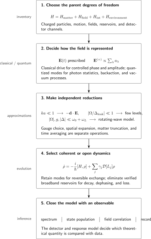
A light–matter calculation is a sequence of declared reductions. Field treatment, spatial expansion, matter truncation, rotating-frame reduction, and reservoir elimination answer different questions and have different validity tests.

The ladder is not a one-way ranking from “classical” to “quantum.” A classical field can be the right controlled input even when the matter is fully quantum. A single quantized mode can be essential in a cavity but inadequate for irreversible free-space emission. An open-system equation can be more realistic than a large closed Hamiltonian if the eliminated reservoir assumptions are verified.

Degrees of freedom before formulas

For each model, inventory:

Sector	Examples	Possible treatment
internal matter	electronic, vibrational, rotational, spin states	exact basis, active subspace, effective levels
center of mass	translation, recoil, trap motion	classical trajectory, wave packet, oscillator modes
applied field	laser, microwave, static bias	prescribed waveform, noisy classical process
retained radiation	cavity, waveguide, pulse mode	quantized bosonic modes
unobserved radiation	free-space vacuum, lossy ports	reservoir spectral density, master equation
material environment	collisions, phonons, solvent, surfaces	stochastic model, bath, explicit modes
detector	counts, homodyne current, transmission	response function, POVM, quantum trajectory

Omitting a sector is a physical claim. For example, replacing center-of-mass motion by a fixed point discards recoil and Doppler effects; replacing the drive by a prescribed field discards source depletion and atom–field entanglement.

Microscopic Electromagnetic Coupling

For nonrelativistic particles with charges $q_a$ and masses $m_a$ in electromagnetic potentials, a standard minimal-coupling Hamiltonian is

$$\begin{aligned} \boldsymbol\pi_a(t) \equiv{}& \mathbf p_a - q_a\mathbf A(\mathbf r_a,t), \\ H ={}& \sum_a \frac{\boldsymbol\pi_a^2(t)}{2m_a} + \sum_a q_a\Phi(\mathbf r_a,t) \\ &+ V_{\mathrm{matter}} + H_{\mathrm{field}}. \end{aligned}$$

$\mathbf A$ and $\Phi$ may be prescribed classical functions or field operators, depending on the model. When they are quantized, $H_{\mathrm{field}}$ is dynamical. When they are prescribed, energy can flow to or from an external source that is not modeled.

Expanding the kinetic term requires Hermitian operator ordering:

$$\begin{aligned} \frac{ \left( \mathbf p-q\mathbf A \right)^2 }{2m} ={}& \frac{\mathbf p^2}{2m} - \frac{q}{2m} \left( \mathbf p\mathbin{\cdot}\mathbf A + \mathbf A\mathbin{\cdot}\mathbf p \right) \\ &+ \frac{q^2\mathbf A^2}{2m}. \end{aligned}$$

The $\mathbf A^2$ term is not decorative. It contributes to diamagnetic response, gauge consistency, strong-coupling physics, and sum-rule relations. Conditions under which a cross term can be simplified depend on the gauge and field dependence.

For spin-$1/2$ matter, the Pauli Hamiltonian also contains magnetic coupling,

$$H_{\mathrm{spin}} = - \boldsymbol\mu\mathbin{\cdot}\mathbf B,$$

with the appropriate magnetic moment and $g$-factor convention. Relativistic corrections generate additional spin–orbit, Darwin, retardation, and multi-particle terms. Nonrelativistic minimal coupling is therefore a parent model within a stated energy regime, not the final form of QED.

Gauge transformations and predictions

Potentials are not unique:

$$\begin{aligned} \mathbf A' &= \mathbf A+\boldsymbol\nabla\chi, \\ \Phi' &= \Phi-\partial_t\chi. \end{aligned}$$

The matter state changes by a position- and time-dependent phase, or by the corresponding unitary transformation in the composite theory. Exact physical predictions are gauge invariant when states, observables, and Hamiltonians are transformed consistently.

Different gauges distribute interaction terms differently. A length-form Hamiltonian may emphasize $-\mathbf d\cdot\mathbf E$, while a velocity-form Hamiltonian emphasizes momentum–vector-potential coupling. Agreement is not guaranteed after an inconsistent basis or level truncation. In ultrastrong-coupling few-level models, how to preserve gauge consistency after truncation remains a technically active literature.

The conservative rule is:

1. choose a parent gauge-covariant theory;
2. transform all operators and states consistently;
3. make approximations in that representation deliberately;
4. test convergence with matter levels and field modes;
5. do not interpret gauge-dependent intermediate partitions as observables.

Spatial and Multipole Approximations

Let $a$ be the characteristic size of the matter wavefunction and $k=2\pi/\lambda$ the field wave number. Expand a field about a reference position $\mathbf R$:

$$\begin{aligned} \mathbf E(\mathbf R+\mathbf r,t) ={}& \mathbf E(\mathbf R,t) \\ &+ \left( \mathbf r\mathbin{\cdot}\boldsymbol\nabla \right) \mathbf E(\mathbf R,t) + \cdots. \end{aligned}$$

The long-wavelength parameter is

$$\eta_{\mathrm{LW}} = ka = \frac{2\pi a}{\lambda}.$$

When $\eta_{\mathrm{LW}}\ll1$, the leading internal electric coupling can be written

$$H_{E1}(t) = - \mathbf d\mathbin{\cdot}\mathbf E(\mathbf R,t),$$

where

$$\mathbf d = \sum_a q_a \left( \mathbf r_a-\mathbf R \right).$$

The next terms include magnetic-dipole and electric-quadrupole couplings, schematically

$$\begin{aligned} H_{\mathrm{int}} ={}& - \mathbf d\mathbin{\cdot}\mathbf E \\ & - \boldsymbol\mu\mathbin{\cdot}\mathbf B \\ & + H_{\mathrm{E2}} + \cdots. \end{aligned}$$

Here $H_{\mathrm{E2}}$ denotes the electric-quadrupole contribution. Quadrupole normalization and sign vary with the definition of the tensor, so a coefficient should never be copied without its convention.

Small spatial parameter does not guarantee E1 dominance

Even when $ka\ll1$, the electric-dipole matrix element can vanish by parity or angular momentum. A nominally higher multipole may then be the leading allowed process. Compare amplitudes, not only powers of $ka$.

Question	Relevant test
Does the field vary across the system?	$ka\ll1$
Is E1 symmetry allowed?	$\langle f
Are gradients important?	compare E2 and E1 matrix elements with $k$ factors
Is magnetic coupling important?	compare M1 and E1 amplitudes for the chosen states
Does center-of-mass motion resolve phase?	compare wave-packet extent and trajectory with $\lambda$

The dipole approximation is a spatial expansion. The two-level and rotating-wave approximations below are independent reductions. Dipole Approximation develops the transition-specific scale tests, origin bookkeeping, and center-of-mass distinction.

Classical Light Driving Quantum Matter

A prescribed electromagnetic field makes the matter Hamiltonian explicitly time dependent. For a real, approximately monochromatic electric field,

$$\mathbf E(t) = \mathcal E_0 \boldsymbol\epsilon \cos \left( \omega_Lt+\phi \right),$$

the electric-dipole interaction is

$$V(t) = - \mathbf d\mathbin{\cdot}\mathbf E(t).$$

The field has a controlled amplitude, polarization, frequency, phase, envelope, propagation vector, and noise process. Calling it classical means these quantities are prescribed rather than operators. Matter remains quantum.

Matrix elements set the drive

For states $|g\rangle$ and $|e\rangle$, define

$$\mathbf d_{eg} = \langle e|\mathbf d|g\rangle.$$

With the real-field convention above, a common on-resonance Rabi-frequency definition is

$$\Omega = - \frac{ \mathcal E_0 \boldsymbol\epsilon\mathbin{\cdot}\mathbf d_{eg} }{\hbar}.$$

The sign and complex phase can be moved by state and field conventions. The measurable rotation rate follows the Hamiltonian convention, so factors of $2$ must be checked at that level.

For a plane wave in vacuum, the cycle-averaged intensity is

$$I = \frac12 c\epsilon_0 \mathcal E_0^2.$$

Thus

$$|\Omega| \propto |\mathbf d_{eg}| \sqrt I.$$

Doubling intensity does not double the Rabi frequency; it multiplies it by $\sqrt2$.

What a prescribed field omits

A classical drive can describe:

• coherent Rabi rotations;
• weak absorption and stimulated emission;
• AC Stark shifts and dynamic polarizability;
• Raman processes under controlled phases;
• pulse shaping and coherent control;
• radiation pressure when field momentum transfer is included.

By itself it does not describe:

• spontaneous emission from vacuum fluctuations;
• photon antibunching or number statistics;
• atom–field entanglement;
• source depletion and quantum backaction;
• vacuum Rabi splitting from a retained mode;
• conditional state changes from individual photon records.

Spontaneous decay can be inserted phenomenologically as a rate, but deriving that rate and its reservoir dependence requires quantized modes. The full physical account lives in Spontaneous Emission.

Weak excitation and coherent cycling

First-order perturbation theory gives a transition amplitude,

$$c_e^{(1)}(t) = - \frac{i}{\hbar} \int_0^t dt'\, e^{i\omega_{eg}t'} \langle e|V(t')|g\rangle.$$

It is reliable while depletion and backaction on the state amplitudes remain small. Near resonance, the amplitude can grow until perturbation theory fails.

A closed two-level model resums that resonant exchange and produces Rabi cycling. For detuning

$$\Delta=\omega_L-\omega_0,$$

one common rotating-frame Hamiltonian is

$$H_{\mathrm{rot}} = \frac{\hbar}{2} \left( - \Delta\sigma_z + \Omega_x\sigma_x + \Omega_y\sigma_y \right).$$

The phase of the classical field determines the transverse direction $(\Omega_x,\Omega_y)$.

Quantized Light Interacting with Matter

For radiation modes labeled by $\lambda$, the free field is

$$H_{\mathrm{field}} = \sum_\lambda \hbar\omega_\lambda \left( a_\lambda^\dagger a_\lambda+\frac12 \right).$$

In a simple quantization volume, the positive-frequency electric field has the form

$$\mathbf E^{(+)}(\mathbf r) = i \sum_\lambda \sqrt{ \frac{ \hbar\omega_\lambda }{ 2\epsilon_0 V } } \, \boldsymbol\epsilon_\lambda a_\lambda e^{i\mathbf k_\lambda\cdot\mathbf r},$$

with normalization modified appropriately for cavities, waveguides, dielectrics, or continuum modes.

The electric-dipole interaction is

$$H_{\mathrm{int}} = - \mathbf d\mathbin{\cdot} \left( \mathbf E^{(+)}+\mathbf E^{(-)} \right).$$

Annihilation and creation operators make field occupation dynamical.

Number factors and vacuum emission

The oscillator matrix elements are

$$\begin{aligned} \langle n-1|a|n\rangle &= \sqrt n, \\ \langle n+1|a^\dagger|n\rangle &= \sqrt{n+1}. \end{aligned}$$

Rates therefore contain $n$ for absorption and $n+1$ for emission. The $+1$ survives at $n=0$ and gives spontaneous emission after coupling to the available vacuum modes and making the continuum approximations that produce irreversibility.

The word vacuum does not mean a classical field of random amplitude. It is the quantum state annihilated by every retained $a_\lambda$, with nonzero field fluctuations and commutators.

One mode: Rabi and Jaynes–Cummings models

After retaining one field mode and two matter levels, a quantum Rabi model can be written

$$\begin{aligned} H_{\mathrm R} ={}& \hbar\omega_c a^\dagger a + \frac{\hbar\omega_0}{2}\sigma_z \\ &+ \hbar g \left( a+a^\dagger \right) \left( \sigma_++\sigma_- \right). \end{aligned}$$

The coupling $g$ contains the dipole matrix element, mode polarization, mode volume, and phase convention.

Near resonance and when counter-rotating terms remain perturbative, the rotating-wave approximation gives the Jaynes–Cummings interaction,

$$\begin{aligned} H_{\mathrm{JC}} ={}& \hbar\omega_c a^\dagger a + \frac{\hbar\omega_0}{2}\sigma_z \\ & + \hbar g \left( a\sigma_+ + a^\dagger\sigma_- \right). \end{aligned}$$

It conserves the excitation number

$$N_{\mathrm{exc}} = a^\dagger a+\sigma_+\sigma_-.$$

In the $n$-excitation manifold, coherent exchange scales as $g\sqrt n$ or $g\sqrt{n+1}$ according to the state pair and convention.

Classical coherent-state limit

A coherent state obeys

$$a|\alpha\rangle = \alpha|\alpha\rangle, \qquad \overline n=|\alpha|^2.$$

When the field remains near a large-amplitude coherent state and the matter-induced change in $\alpha$ is negligible, replacing $a$ by $\alpha$ reduces the quantized coupling to a semiclassical drive. The corresponding Rabi scale is proportional to

$$g|\alpha| = g\sqrt{\overline n}.$$

This is a controlled correspondence, not a statement that every bright quantum field is classical. Squeezing, number states, entanglement, conditional detection, and nonlinear backaction can remain quantum at large mean occupation.

Many modes and irreversibility

A closed atom plus a finite set of lossless modes evolves unitarily and can return excitation to the atom. Exponential spontaneous decay emerges after coupling to a sufficiently broad mode continuum and neglecting memory and recurrence over the observation time.

A schematic system–bath Hamiltonian is

$$\begin{aligned} H ={}& H_S + \sum_k \hbar\omega_k b_k^\dagger b_k \\ & + \hbar \sum_k \left( g_k L^\dagger b_k + g_k^*L b_k^\dagger \right). \end{aligned}$$

The spectral density

$$J(\omega) = \sum_k |g_k|^2 \delta(\omega-\omega_k)$$

controls decay, shifts, and memory. Free space, a cavity, a waveguide, a photonic crystal, and a nearby surface have different $J(\omega)$ and therefore different radiative dynamics.

Minimal Coupling and Approximation Ledger

The common approximations are independent. Passing one test does not imply the others.

Reduction	Small parameter or test	What is discarded
nonrelativistic matter	binding and kinetic energies $\ll mc^2$	pair creation and relativistic corrections
long wavelength	$ka\ll1$	spatial field variation across internal state
electric dipole	E1 allowed and dominant	M1, E2, and higher multipoles
prescribed field	source backaction negligible	field depletion, entanglement, photon statistics
two-level truncation	drive and bandwidth small versus leakage gaps	off-resonant matter levels
rotating-wave approximation	$	\Delta
Markov reservoir	bath correlation time $\tau_B\ll\tau_S$	memory and recurrence
secular master equation	distinct Bohr frequencies separated relative to damping	coherence between unresolved transition sectors
weak-coupling decay	radiative coupling perturbative	nonperturbative dressing and bound states
fixed center of mass	recoil, Doppler, and motional entanglement negligible	translational dynamics

Order of approximations matters

Gauge transformation, matter truncation, field-mode truncation, and the rotating-wave approximation need not commute. For example:

1. transform the full Hamiltonian and then truncate;
2. truncate first and then transform inside the reduced space;

can produce different effective operators. Agreement improves only when the reduced construction preserves the parent theory’s constraints or when convergence is demonstrated.

The same warning applies to eliminating a far-detuned level before or after including decay: coherent Stark shifts and dissipative scattering can be lost if the elimination is incomplete.

A practical scale vector

Before solving, collect

$$\mathcal S = \left\{ \begin{array}{c} \omega_0,\, \omega_L,\, |\Delta|,\, |\Omega|,\, g,\, \Gamma, \\ \gamma_\phi,\, \kappa,\, \Delta_{\mathrm{leak}},\, \tau_{\mathrm p}^{-1} \end{array} \right\}.$$

Here $\kappa$ is a retained-mode linewidth, $\Delta_{\mathrm{leak}}$ the nearest unwanted matter detuning, and $\tau_{\mathrm p}$ a pulse timescale. Ratios among these scales decide the model:

$$\begin{gathered} \frac{|\Omega|}{\Delta_{\mathrm{leak}}}, \qquad \frac{g}{\omega_0}, \qquad \frac{\Gamma}{|\Omega|} \\ \qquad \frac{\kappa}{g}, \qquad \frac{1}{\omega_0\tau_{\mathrm p}}. \end{gathered}$$

No single label such as “weak,” “fast,” or “strong coupling” replaces these ratios.

Two-Level Systems as the Basic Model

Choose two matter eigenstates $|g\rangle$ and $|e\rangle$ with splitting $\hbar\omega_0$. Projection gives

$$H_0 = \frac{\hbar\omega_0}{2}\sigma_z + \text{constant}.$$

The projected dipole operator is

$$P\mathbf dP = \mathbf d_{eg}\sigma_+ + \mathbf d_{ge}\sigma_- + \mathbf d_{\mathrm{diag}},$$

where

$$P = |g\rangle\langle g| + |e\rangle\langle e|.$$

Diagonal dipoles may vanish by parity or symmetry, but they are not absent for every effective two-state system.

Validity of the truncation

A two-level model is justified when:

• the drive spectrum is concentrated near one transition;
• other states are detuned compared with their driven matrix elements;
• off-resonant AC Stark shifts are included or negligible;
• pulse edges do not contain substantial high-frequency leakage;
• spontaneous decay does not populate relevant states outside the pair;
• selection rules and polarization suppress unwanted channels;
• the desired accuracy is coarser than residual multilevel corrections.

For an unwanted state $|r\rangle$ with detuning $\Delta_r$ and coupling $\Omega_r$, a rough coherent leakage scale is

$$P_r \sim \left| \frac{\Omega_r}{\Delta_r} \right|^2$$

away from resonance and for a sufficiently smooth pulse. This estimate misses spectral side lobes, multiphoton resonance, and interference among paths, but it is a useful first audit.

Detuning and rotating frames

Detuning conventions differ. This page uses

$$\Delta=\omega_L-\omega_0.$$

Other pages or books may use the negative. A rotating-frame Hamiltonian must be read together with that definition.

The rotating frame removes a known carrier phase from the state description. It does not physically eliminate the optical frequency. Terms discarded by the rotating-wave approximation can produce Bloch–Siegert shifts, multiphoton processes, and ultrastrong-coupling effects.

Dressed states

Diagonalizing the driven or atom–mode Hamiltonian produces dressed states: eigenstates of the coupled model rather than bare matter or field states. This language explains avoided crossings, Autler–Townes splitting, vacuum Rabi splitting, and adiabatic transfer.

“Dressed” is model-relative. A state dressed by a classical periodic drive belongs naturally to Floquet or rotating-frame theory; a state dressed by a quantized mode can be atom–field entangled. Similar spectra do not make the underlying states identical. Dressed States develops the mixing-angle transformation, photon-number manifolds, adiabatic preparation, and Floquet dictionary. Autler–Townes Splitting then develops the weak-probe spectrum, pole criterion, line strengths, and distinction from interference-induced transparency. Electromagnetically Induced Transparency develops the complementary dark-state susceptibility, slow-light, and optical-memory limits.

Coherent Versus Dissipative Dynamics

Closed composite dynamics obey

$$\frac{d\rho}{dt} = - \frac{i}{\hbar} [H,\rho].$$

This includes coherent population transfer, phase accumulation, atom–field entanglement, collapse and revival in few-mode models, and reversible exchange. It does not by itself produce irreversible loss of information.

After eliminating unobserved reservoirs under Markovian conditions, a driven two-level atom and lossy mode may obey

$$\begin{aligned} \dot\rho ={}& - \frac{i}{\hbar} [H,\rho] + \Gamma\mathcal D[\sigma_-]\rho \\ &+ \frac{\gamma_\phi}{2} \mathcal D[\sigma_z]\rho + \kappa\mathcal D[a]\rho, \end{aligned}$$

where

$$\mathcal D[L]\rho = L\rho L^\dagger - \frac12 \left\{ L^\dagger L,\rho \right\}.$$

$\Gamma$ is matter population decay, $\gamma_\phi$ is pure dephasing, and $\kappa$ is retained-mode energy decay in this convention.

Timescale competition

The qualitative regime depends on competing rates:

Regime	Typical hierarchy	Behavior
weak excitation	$	\Omega
coherent drive	$	\Omega
saturated response	drive competes with relaxation	power broadening and bounded population
strong cavity coupling	coherent $g$ exceeds relevant losses	resolved exchange or normal-mode splitting
bad-cavity or Purcell regime	cavity loss fast but structured density of states important	modified irreversible emission
non-Markovian reservoir	bath memory not short	time-dependent rates, revivals, bound-state effects

These labels need quantitative conventions. In cavity QED, one often defines a cooperativity of the form

$$C = \frac{4g^2}{\kappa\Gamma},$$

but factors vary with whether $\kappa$ and $\Gamma$ denote energy, amplitude, population, or half widths. State the dynamical equations before quoting $C$.

Dissipation is not failed coherence

Radiative decay is coherent in the full matter-plus-field state. It appears irreversible for the matter subsystem when emitted modes are unobserved and do not return. Dephasing likewise can arise from entanglement with unresolved environmental degrees of freedom.

This distinction prevents two mistakes:

• adding a non-Hermitian energy by hand without specifying the missing jumps or normalization;
• claiming that a unitary atom-plus-one-mode model derives free-space exponential decay.

Monitoring changes the description

An unconditional master equation averages over all detector records. If fluorescence photons, homodyne current, or transmitted photons are monitored, the conditioned state follows a stochastic quantum trajectory.

The average over records recovers the master equation:

$$\rho(t) = \mathbb E \left[ \rho_c(t) \right].$$

The detector efficiency and response determine how much information is available. A photon count is not merely evidence that the atom “was excited”; it is an outcome of a coupled preparation, dynamics, collection, and measurement model.

Spectroscopy, Control, and Measurement

The same Hamiltonian serves different experimental goals.

Spectroscopy

Spectroscopy usually scans frequency, field, delay, or momentum and asks which matter parameters explain the response. In a weak-drive limit, line positions and intensities can be related to energy differences and matrix elements. At stronger drive, saturation, AC Stark shifts, Autler–Townes splitting, power broadening, and optical pumping become part of the spectrum.

The inference chain is

$$\begin{gathered} \text{prepared matter} \\ \text{with a characterized field} \\ \downarrow \\ \text{light–matter dynamics} \\ \downarrow \\ \text{emitted or transmitted light} \\ \text{or a state-resolved record} \\ \downarrow \\ \text{line and response model} \\ \downarrow \\ \text{energies and matrix elements} \\ \text{rates and shifts}. \end{gathered}$$

The Spectroscopy Overview owns this measurement language in detail.

Coherent control

Control chooses field amplitude, phase, polarization, frequency, and timing to implement a target map. For a two-level system, the pulse area is

$$\Theta = \int dt\,\Omega(t).$$

On resonance in the ideal rotating-wave model, $\Theta=\pi$ gives inversion and $\Theta=\pi/2$ gives an equal-population superposition, up to phase conventions. Real control must include:

• detuning and dynamic phase;
• finite pulse bandwidth;
• leakage to other levels;
• spatial intensity variation;
• oscillator phase noise;
• spontaneous scattering and dephasing;
• calibration and detector errors.

Adiabatic passage, Raman transfer, and dark-state protocols trade simple pulse area for eigenstate following and interference. Their advantages are conditional on adiabaticity, two-photon resonance, and loss from intermediate states.

Measurement and backaction

Absorption, fluorescence, dispersive phase, cavity transmission, and photoionization reveal different observables. A detector model can be written schematically as

$$p(m) = \operatorname{Tr} \left( E_m\rho_{\mathrm{out}} \right),$$

where $E_m$ is a POVM element for outcome $m$. The outgoing state $\rho_{\mathrm{out}}$ already includes the light–matter interaction and any unobserved loss.

Dispersive probing can reduce population transfer while still entangling light and matter. Calling it “non-destructive” means the relevant observable and disturbance are controlled, not that backaction vanishes.

Three objectives, three failure tests

Objective	Minimal useful model	Main failure test
locate weak line	perturbative drive plus line shape	depletion, unresolved structure, field shifts
implement gate or transfer	coherent few-level dynamics	leakage, phase error, decoherence
predict fluorescence	driven open-system model	non-Markov memory, detector response, extra levels
resolve photon statistics	quantized field plus measurement	semiclassical replacement loses correlations
infer dipole matrix element	calibrated field and response	polarization, degeneracy, intensity calibration
engineer spontaneous emission	structured reservoir model	free-space rate or one-mode model inadequate

Worked Examples

Long-wavelength estimate for an atom

Take an internal length scale

$$a=0.10\ \mathrm{nm}$$

and light of wavelength

$$\lambda=500\ \mathrm{nm}.$$

Then

$$\begin{aligned} ka &= \frac{2\pi a}{\lambda} \\ &= \frac{ 2\pi(0.10\ \mathrm{nm}) }{ 500\ \mathrm{nm} } \\ &\simeq 1.26\times10^{-3}. \end{aligned}$$

Spatial variation across the atom is small. An E1-forbidden transition can still require M1 or E2 coupling, so this number does not alone decide the leading amplitude.

Rabi frequency from intensity

Let

$$I=1.0\ \mathrm{mW\,cm^{-2}} = 10\ \mathrm{W\,m^{-2}},$$

and assume a polarization-projected dipole magnitude

$$|d_{eg}|=3ea_0.$$

The field amplitude is

$$\begin{aligned} \mathcal E_0 &= \sqrt{ \frac{2I}{c\epsilon_0} } \\ &\simeq 86.8\ \mathrm{V\,m^{-1}}. \end{aligned}$$

Using

$$3ea_0 \simeq 2.54\times10^{-29}\ \mathrm{C\,m},$$

the Rabi scale is

$$\begin{aligned} |\Omega| &= \frac{ |d_{eg}|\mathcal E_0 }{\hbar} \\ &\simeq 2.09\times10^7\ \mathrm{s^{-1}} \\ &\simeq 2\pi\times3.33\ \mathrm{MHz}. \end{aligned}$$

This ideal estimate assumes the quoted intensity occurs at the particle, polarization is perfectly projected onto the transition, and the real-field Rabi convention used above applies.

Leakage audit

Suppose the desired drive has

$$\frac{\Omega}{2\pi} = 1.0\ \mathrm{MHz},$$

and an unwanted level has comparable matrix element but detuning

$$\frac{\Delta_r}{2\pi} = 100\ \mathrm{MHz}.$$

The rough off-resonant population scale is

$$P_r \sim \left( \frac{\Omega}{\Delta_r} \right)^2 = 10^{-4}.$$

That may be negligible for a percent-level spectrum and unacceptable for a high-fidelity gate. Pulse shape, intermediate Stark shifts, and coherent return can change the final leakage.

Quantum versus classical amplitude

For a single quantized mode in a coherent state with

$$\overline n=10^6,$$

the semiclassical coupling scale is

$$g\sqrt{\overline n} = 10^3g.$$

Absorbing one photon changes the field amplitude by a relative amount of order $1/\overline n$ in photon number and $1/(2\overline n)$ in $\sqrt n$. Backaction on a bright coherent drive can therefore be tiny even though the coupling event is quantized. For a number state with the same $\overline n$, phase and fluctuations differ; mean occupation alone does not define the classical limit.

Choosing a Model

Start from the observable

Observable	First model to try	Add when needed
weak absorption spectrum	classical field plus perturbative matter	multilevel structure, propagation, open dynamics
Rabi population trace	driven two-level Hamiltonian	decay, leakage, spatial averaging
spontaneous lifetime	quantized continuum and golden rule	structured reservoir, non-Markov memory
cavity transmission	quantized retained mode plus input–output loss	multilevel emitters, technical noise
photon antibunching	quantum source, modes, and detector	timing response, background counts
AC Stark shift	off-resonant classical drive	multilevel dynamic response, tensor structure
Raman transfer	at least three matter levels and two fields	spontaneous scattering, differential shifts
radiation pressure	internal state plus center-of-mass momentum	diffusion, recoil, multibeam geometry

Record the approximation ledger

For every result, state:

1. the retained matter levels and motional modes;
2. whether the applied field is classical or quantized;
3. the gauge and interaction representation;
4. the spatial order in $ka$;
5. whether counter-rotating and $\mathbf A^2$-related terms are retained;
6. the reservoir and Markov assumptions;
7. the drive, detuning, leakage, and decay scales;
8. the measured observable and detector model;
9. the convergence or limiting-case checks.

Limiting-case checks

A useful model should reduce correctly when:

• field amplitude tends to zero;
• detuning becomes large;
• decay rates vanish;
• mode occupation becomes large and coherent;
• cavity coupling tends to zero;
• the nearest unwanted level is moved far away;
• $ka$ tends to zero;
• detector efficiency tends to zero or one.

These checks catch missing factors, incorrect rotating-frame signs, unphysical gain, and inconsistent truncations.

Common Mistakes

• Calling light classical and matter quantum a contradiction. A prescribed classical field is an approximation for the source, not for the matter state.
• Using $-\mathbf d\cdot\mathbf E$ without stating the long-wavelength and representation assumptions.
• Dropping $\mathbf A^2$ before deciding the gauge, basis, and coupling regime.
• Assuming gauge equivalence survives arbitrary few-level truncation.
• Treating $ka\ll1$ as proof that an E1 matrix element is nonzero.
• Using a two-level model because only two levels are plotted. Spectral isolation and leakage must be checked.
• Mixing detuning and Rabi-frequency conventions. Read definitions from the Hamiltonian.
• Calling rotating-wave terms “energy conserving” in an absolute sense. They conserve excitation number in the reduced near-resonant model.
• Deriving irreversible decay from one lossless mode. A finite closed model can exchange and revive.
• Adding decay to amplitudes without jump terms when probabilities and emitted records matter.
• Treating spontaneous emission as an intrinsic number independent of electromagnetic environment.
• Equating a bright field with a coherent state. Thermal, squeezed, and number states can be bright without the same phase-space structure.
• Calling dispersive measurement backaction-free.
• Using strong-coupling labels without stating $g$, $\kappa$, $\Gamma$, and their linewidth conventions.

Exercises

1. Expand minimal coupling

Expand $(\mathbf p-q\mathbf A)^2/(2m)$ without assuming that $\mathbf p$ and $\mathbf A(\mathbf r,t)$ commute. Why is symmetrization necessary?

Solution

Direct multiplication gives

$$\begin{aligned} T \equiv{}& \frac{ \left( \mathbf p-q\mathbf A \right)^2 }{2m}, \\ T ={}& \frac{\mathbf p^2}{2m} - \frac{q}{2m} \left( \mathbf p\mathbin{\cdot}\mathbf A + \mathbf A\mathbin{\cdot}\mathbf p \right) \\ &+ \frac{q^2\mathbf A^2}{2m}. \end{aligned}$$

In position representation, $\mathbf p=-i\hbar\boldsymbol\nabla$ acts on both $\mathbf A$ and the state to its right. Replacing the cross term by $-(q/m)\mathbf A\cdot\mathbf p$ without the conditions that permit that simplification can lose a derivative term and spoil Hermiticity. The symmetrized form is manifestly Hermitian for real classical $\mathbf A$ or a Hermitian field operator.

2. Test the dipole approximation

A molecule has spatial extent $a=0.50\ \mathrm{nm}$. Compute $ka$ for $\lambda=10\ \mathrm{\mu m}$ infrared light and for $\lambda=0.10\ \mathrm{nm}$ X-rays. Interpret the result.

Solution

For infrared light,

$$\begin{aligned} ka_{\mathrm{IR}} &= \frac{ 2\pi(0.50\ \mathrm{nm}) }{ 10^4\ \mathrm{nm} } \\ &\simeq 3.14\times10^{-4}. \end{aligned}$$

The field is nearly uniform over the molecule.

For the X-rays,

$$\begin{aligned} ka_{\mathrm X} &= \frac{ 2\pi(0.50\ \mathrm{nm}) }{ 0.10\ \mathrm{nm} } \\ &\simeq 31.4. \end{aligned}$$

The long-wavelength expansion is not controlled for the full molecular extent. Spatial phase, momentum transfer, and higher multipoles must be retained. A localized core orbital can have a smaller effective $a$, so the relevant size depends on the transition density rather than only the geometric molecule.

3. Intensity scaling

If a resonant Rabi frequency is $2\pi\times1.0\ \mathrm{MHz}$ at intensity $I_0$, what is it at $9I_0$ with all else unchanged? How does the $\pi$-pulse time change?

Solution

Since $\mathcal E_0\propto\sqrt I$ and $|\Omega|\propto\mathcal E_0$,

$$\Omega(9I_0) = 3\Omega(I_0) = 2\pi\times3.0\ \mathrm{MHz}.$$

With the convention $t_\pi=\pi/|\Omega|$, the pulse time is reduced by a factor of three. This assumes no saturation-induced change of the effective model, no AC Stark detuning, and no intensity-dependent loss.

4. Recover the occupation factors

Show that the squared matrix elements for $|g,n\rangle\to|e,n-1\rangle$ and $|e,n\rangle\to|g,n+1\rangle$ are proportional to $n$ and $n+1$, respectively.

Solution

In the rotating-wave interaction, absorption contains $a\sigma_+$:

$$\begin{aligned} \langle e,n-1| a\sigma_+ |g,n\rangle &= \langle n-1|a|n\rangle \\ &= \sqrt n. \end{aligned}$$

Its squared magnitude is $n$.

Emission contains $a^\dagger\sigma_-$:

$$\begin{aligned} \langle g,n+1| a^\dagger\sigma_- |e,n\rangle &= \langle n+1|a^\dagger|n\rangle \\ &= \sqrt{n+1}. \end{aligned}$$

Its squared magnitude is $n+1$. At $n=0$, absorption vanishes while emission retains the vacuum contribution.

5. Verify Jaynes–Cummings excitation conservation

For

$$H_{\mathrm{int}} = \hbar g \left( a\sigma_+ + a^\dagger\sigma_- \right),$$

show that

$$N_{\mathrm{exc}} = a^\dagger a+\sigma_+\sigma_-$$

commutes with $H_{\mathrm{int}}$.

Solution

Use

$$[a^\dagger a,a]=-a, \qquad [a^\dagger a,a^\dagger]=a^\dagger,$$

and

$$\begin{aligned} [\sigma_+\sigma_-,\sigma_+] &= \sigma_+, \\ [\sigma_+\sigma_-,\sigma_-] &= -\sigma_-. \end{aligned}$$

Then

$$\begin{aligned} [N_{\mathrm{exc}},a\sigma_+] &= (-a)\sigma_+ + a\sigma_+ = 0, \\ [N_{\mathrm{exc}},a^\dagger\sigma_-] &= a^\dagger\sigma_- - a^\dagger\sigma_- = 0. \end{aligned}$$

Therefore

$$[N_{\mathrm{exc}},H_{\mathrm{int}}]=0.$$

The counter-rotating terms $a\sigma_-$ and $a^\dagger\sigma_+$ do not conserve this excitation number.

6. Audit a two-level truncation

A desired transition is driven with $\Omega/2\pi=2\ \mathrm{MHz}$. Two unwanted states have projected couplings $0.3\Omega$ and $1.2\Omega$, at detunings $40\ \mathrm{MHz}$ and $300\ \mathrm{MHz}$, respectively. Estimate their separate leakage scales.

Solution

For the first state,

$$\begin{aligned} P_1 &\sim \left( \frac{ 0.3(2\ \mathrm{MHz}) }{ 40\ \mathrm{MHz} } \right)^2 \\ &= 2.25\times10^{-4}. \end{aligned}$$

For the second,

$$\begin{aligned} P_2 &\sim \left( \frac{ 1.2(2\ \mathrm{MHz}) }{ 300\ \mathrm{MHz} } \right)^2 \\ &= 6.4\times10^{-5}. \end{aligned}$$

The more strongly coupled state leaks less because it is much farther detuned. These estimates do not include pulse-spectrum side lobes, interference, Stark shifts, or decay. They rank which channels deserve a full multilevel simulation.

7. Coherent or dissipative?

A driven transition has

$$\frac{\Omega}{2\pi}=5\ \mathrm{MHz}, \qquad \Gamma^{-1}=30\ \mathrm{ns}.$$

Estimate how many resonant Rabi periods fit within one population lifetime. Would you expect clean oscillations?

Solution

The Rabi period is

$$T_R = \frac{2\pi}{\Omega} = \frac{1}{5\ \mathrm{MHz}} = 200\ \mathrm{ns}.$$

The lifetime-to-period ratio is

$$\frac{\Gamma^{-1}}{T_R} = \frac{30\ \mathrm{ns}}{200\ \mathrm{ns}} = 0.15.$$

Population decays substantially before one Rabi cycle is completed, so clean oscillations are not expected. The optical Bloch equations, including dephasing and actual pulse duration, are more appropriate than a closed Rabi formula.

8. Design the minimum model

An experiment drives a trapped ion with a laser and records time-tagged fluorescence photons while resolving motional sidebands. List the minimum degrees of freedom and approximations needed for a model that predicts both internal populations and the photon record.

Solution

A minimum defensible model includes:

1. the relevant internal levels, including any shelving or decay branches;
2. quantized trap motion for each resolved motional mode;
3. the laser as a characterized classical drive, including wave vector, phase, detuning, and intensity;
4. position-dependent coupling $e^{i\mathbf k\cdot\mathbf x}$, expanded in the Lamb–Dicke parameter only if that parameter is small;
5. spontaneous-emission jump operators with branching ratios and recoil;
6. any relevant laser phase noise, magnetic noise, or motional heating;
7. a photon-counting unraveling or measurement model with collection efficiency, dark counts, timing response, and dead time.

The rotating-wave, two-level, Lamb–Dicke, Markov, and secular approximations must each be checked. An unconditional master equation predicts averaged populations and mean fluorescence, but a time-tagged photon record requires a conditioned trajectory or equivalent counting-statistics calculation.

Further Connections

• Laser Nomenclature fixes the real-field Rabi-frequency, laser-minus-transition detuning, local intensity, and saturation conventions used when a laser drives matter.
• Dipole Approximation gives the controlled spatial reduction behind the E1 interaction used throughout this overview.
• Spectroscopy Overview treats spectra as preparation–interaction–detection inference.
• Transition Rates distinguishes finite-pulse probabilities, rates, and detector channels.
• Einstein Coefficients connects absorption, stimulated emission, spontaneous emission, and equilibrium radiation.
• Atomic Selection Rules applies multipole and angular-momentum structure to atoms.
• Kubo Formula supplies the response-function viewpoint for weak fields.
• Rotating-Wave Approximation develops the controlled averaging behind near-resonant effective Hamiltonians.
• Rabi and Ramsey Control treats pulse calibration in the presence of relaxation and dephasing.
• Rabi Oscillations connects coupling conventions to population traces, pulse areas, chevrons, and experimental model checks.
• Ramsey Interferometry develops separated-pulse fringes, detuning estimators, and atomic-clock error signals.
• Optical Bloch Equations connects coherent drive and dissipation to saturation, fluorescence counts, and power-broadened lines.
• Autler–Townes Splitting explains when a strong control turns one weak-probe resonance into a resolvable dressed doublet.
• Electromagnetically Induced Transparency develops dark-state interference, transparent bandwidth, dispersive delay, and reversible spin-wave storage.
• STIRAP develops counterintuitive pulse ordering, dark-state adiabatic following, detuning and loss limits, and coherent population transfer.
• Radiation Pressure derives the saturated scattering force, Doppler dependence, recoil diffusion, and its distinction from conservative dipole forces.
• Spontaneous Emission derives the vacuum-continuum decay behind the radiative rate and explains its angular, spectral, recoil, and environment dependence.
• Stimulated Emission develops Bose enhancement, population inversion, propagation gain, saturation, amplifier noise, and the laser-threshold connection.
• AC Stark Shift develops off-resonant light shifts, virtual admixture, trap potentials, and differential clock systematics.
• Dynamic Polarizability builds frequency-dependent response from atomic structure and locates resonances, tune-out zeros, and magic trapping conditions.
• Dressed States diagonalizes coupled matter–field models and separates rotating-frame, Floquet, and physical atom–photon meanings.
• Input–Output Theory connects retained cavities to propagating measured fields.
• Photon Counting owns the conditioned jump-record description.

References

• C. Cohen-Tannoudji, J. Dupont-Roc, and G. Grynberg, Photons and Atoms: Introduction to Quantum Electrodynamics, Wiley, 1989 — canonical, multipolar, and quantized-field formulations.
• C. Cohen-Tannoudji, J. Dupont-Roc, and G. Grynberg, Atom–Photon Interactions: Basic Processes and Applications, Wiley, 1992 — coherent excitation, radiative processes, dressed atoms, and effective Hamiltonians.
• L. Allen and J. H. Eberly, Optical Resonance and Two-Level Atoms, Dover, 1987 — semiclassical two-state dynamics and optical Bloch equations.
• B. W. Shore, The Theory of Coherent Atomic Excitation, Wiley, 1990 — multilevel coherent dynamics, pulse methods, and approximation control.
• R. Loudon, The Quantum Theory of Light, 3rd ed., Oxford University Press, 2000 — field quantization, photon statistics, and radiative processes.
• L. Mandel and E. Wolf, Optical Coherence and Quantum Optics, Cambridge University Press, 1995 — classical and quantum coherence, photodetection, and propagation.
• M. O. Scully and M. S. Zubairy, Quantum Optics, Cambridge University Press, 1997 — few-level atoms, quantized modes, coherence, and dissipation.
• I. I. Rabi, “Space Quantization in a Gyrating Magnetic Field,” Physical Review 51, 652–654 (1937), doi:10.1103/PhysRev.51.652 — coherent near-resonant spin driving.
• E. T. Jaynes and F. W. Cummings, “Comparison of Quantum and Semiclassical Radiation Theories with Application to the Beam Maser,” Proceedings of the IEEE 51, 89–109 (1963), doi:10.1109/JRPROC.1963.1664 — one-mode matter–radiation exchange and the quantum–semiclassical comparison.
• E. A. Power and S. Zienau, “Coulomb Gauge in Non-Relativistic Quantum Electro-Dynamics and the Shape of Spectral Lines,” Philosophical Transactions of the Royal Society A 251, 427–454 (1959), doi:10.1098/rsta.1959.0008 — multipolar transformation and interaction representation.
• R. J. Glauber, “Coherent and Incoherent States of the Radiation Field,” Physical Review 131, 2766–2788 (1963), doi:10.1103/PhysRev.131.2766 — coherent states and optical coherence.
• H. J. Carmichael, Statistical Methods in Quantum Optics 1, Springer, 1999, doi:10.1007/978-3-662-03875-8 — master equations, regression, and photon-counting trajectories.
• A. F. Kockum, A. Miranowicz, S. De Liberato, S. Savasta, and F. Nori, “Ultrastrong Coupling between Light and Matter,” Nature Reviews Physics 1, 19–40 (2019), doi:10.1038/s42254-018-0006-2 — regimes where rotating-wave, mode, and truncation assumptions become delicate.
• O. Di Stefano et al., “Resolution of Gauge Ambiguities in Ultrastrong-Coupling Cavity Quantum Electrodynamics,” Nature Physics 15, 803–808 (2019), doi:10.1038/s41567-019-0534-4; A. Stokes and A. Nazir, “Gauge Non-Invariance Due to Material Truncation in Ultrastrong-Coupling Quantum Electrodynamics,” Nature Physics 20, 376–378 (2024), doi:10.1038/s41567-023-02155-8 — active debate over gauge-consistent finite-level constructions.