Rabi Oscillations: First Encounter

Rabi oscillations are coherent population oscillations in a driven two-level system. If a drive is close to the transition frequency and the two-level approximation remains valid, the system can cycle between the lower and upper states instead of making a one-way transition.

This page gives the standard first formula and its interpretation. Detailed spectroscopy, pulse shaping, light-matter coupling, rotating-wave error estimates, and open-system damping belong to later pages; the driven dissipative two-level model is treated in Optical Bloch Equations.

Two-Level Atom owns the preceding AMO step: selecting two physical states from a multilevel spectrum, projecting the drive, and auditing spectator leakage and frame conventions. This page assumes that reduction and solves the resulting closed model.

Rabi Oscillations continues in the experimental direction: it maps the coupling to field intensity, defines pulse areas, and shows how traces, chevrons, readout errors, decoherence, and multilevel effects are diagnosed.

Driven Two-Level Model

Start with an undriven two-level Hamiltonian

$$H_0 = \frac{\hbar\omega_0}{2}\sigma_z,$$

where $\omega_0$ is the transition angular frequency. Add a classical sinusoidal drive that couples the two basis states:

$$V(t) = \hbar\Omega\cos(\omega t)\sigma_x.$$

Here $\omega$ is the drive angular frequency, and $\Omega$ sets the drive strength in this convention. Different books place factors of $2$ in different parts of the definition of $\Omega$, so always check the Hamiltonian before comparing Rabi frequencies.

The full Hamiltonian is

$$H(t) = \frac{\hbar\omega_0}{2}\sigma_z + \hbar\Omega\cos(\omega t)\sigma_x.$$

Near resonance and for a weak drive, the fast counter-rotating part can often be dropped. This is the Rotating-Wave Approximation, not an exact identity.

Effective Hamiltonian

In a frame rotating with the drive, the leading effective Hamiltonian has the form

$$H_{\mathrm{eff}} = \frac{\hbar}{2} \left( \Delta\sigma_z+\Omega\sigma_x \right),$$

where the detuning is

$$\Delta=\omega_0-\omega.$$

This is just a time-independent Pauli-vector Hamiltonian with effective field

$$\mathbf b_{\mathrm{eff}} = \frac{\hbar}{2} (\Omega,0,\Delta).$$

The problem has therefore become the precession of a two-level state around a fixed effective field in the rotating frame.

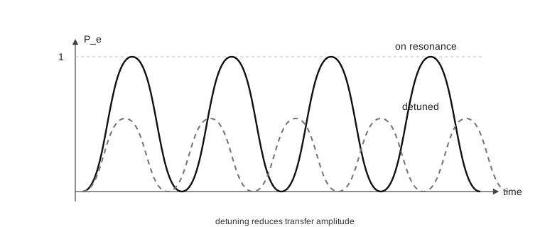
On resonance, a driven two-level system can transfer population completely between the two levels. Detuning tilts the effective field and reduces the maximum transition probability.

Rabi Formula

Suppose the system starts in the lower state of $\sigma_z$, written $\lvert g\rangle$. Under $H_{\mathrm{eff}}$, the probability of finding the upper state $\lvert e\rangle$ at time $t$ is

$$P_e(t) = \frac{\Omega^2}{\Omega_R^2} \sin^2 \left( \frac{\Omega_R t}{2} \right),$$

where the generalized Rabi frequency is

$$\Omega_R = \sqrt{\Omega^2+\Delta^2}.$$

The maximum transition probability is

$$P_{e,\mathrm{max}} = \frac{\Omega^2}{\Omega^2+\Delta^2}.$$

Thus detuning does two things at once: it increases the oscillation frequency from $\Omega$ to $\Omega_R$, and it suppresses the oscillation amplitude.

Exact Resonance

On resonance,

$$\Delta=0,$$

so

$$\Omega_R=\Omega$$

and

$$P_e(t) = \sin^2 \left( \frac{\Omega t}{2} \right).$$

The first complete transfer occurs at

$$t_\pi = \frac{\pi}{\Omega}.$$

This is called a $\pi$ pulse in this convention. A pulse of duration

$$t_{\pi/2} = \frac{\pi}{2\Omega}$$

creates an equal-population superposition, up to phase conventions.

Bloch-Sphere Picture

In the rotating frame, the effective field is $(\Omega,0,\Delta)$. On resonance, this field lies along the $x$ axis, so an initial south-pole state rotates through the equator and reaches the north pole.

For nonzero detuning, the field is tilted toward $z$. The Bloch vector rotates around that tilted axis. Because the rotation axis is no longer perpendicular to the initial state, the trajectory does not reach the north pole; the excited-state probability oscillates with reduced amplitude.

The Bloch-sphere page explains the geometry of this rotation in Bloch Sphere: Wave-Mechanics Perspective.

Relation To Perturbation Theory

In weak first-order transition theory, a resonant harmonic drive produces transition probability that initially grows like $t^2$. The exact two-level result agrees at short times:

$$P_e(t) \approx \frac{\Omega^2t^2}{4} \qquad (\Delta=0,\ \Omega t\ll1).$$

But the exact two-level dynamics do not grow forever. Population returns to the initial state because the system is closed and coherent. This is why Rabi oscillations are not the same thing as irreversible absorption.

The weak-drive transition-amplitude viewpoint is developed in Harmonic Perturbations. Resonant Driving gives the finite-pulse linewidth and shows why the short-time polynomial ceases to be valid when $\Omega t$ becomes order one. Rabi Formula in the Weak-Drive Limit derives the matching expansion and its first correction.

Physical Examples

Rabi oscillations appear in many controlled two-level settings:

• spin resonance in magnetic fields;
• two selected atomic or molecular levels driven by radiation;
• superconducting or semiconductor qubits under microwave control;
• trapped-ion internal states;
• quantum-dot charge or spin states.

In each case, the symbols $\Omega$ and $\Delta$ must be translated into the physical drive amplitude, matrix element, and detuning. A strong drive may invalidate the two-level approximation or require corrections beyond the rotating-wave approximation.

Common Mistakes

• Treating $\Omega$ as a universal number independent of convention and matrix element.
• Forgetting detuning; an off-resonant drive may oscillate faster but transfer less population.
• Confusing coherent Rabi cycling with irreversible decay or absorption.
• Applying the rotating-wave approximation without checking weak-drive and near-resonance conditions.
• Ignoring other levels that the same drive can couple to.
• Calling every driven oscillation a Rabi oscillation without identifying the two-state truncation.

Where This Is Used

• Pauli-Matrix Hamiltonians gives the effective-field notation.
• Bloch Sphere: Wave-Mechanics Perspective gives the rotation picture.
• Spin-1/2 as a Canonical System: First Encounter gives the spin-resonance dictionary for static and transverse magnetic fields.
• Harmonic Perturbations gives the weak-drive transition-amplitude limit.
• Resonant Driving separates Fourier width, detuning, and resonant perturbative breakdown.
• Rabi Oscillations connects the closed solution to AMO coupling calibration, pulse areas, measured traces, and chevrons.
• Rabi Formula in the Weak-Drive Limit gives the controlled asymptotic match and error terms.
• Rotating-Wave Approximation gives the method that produces the effective Hamiltonian.
• Time-Dependent Hamiltonians explains the general formal issue of explicitly time-dependent generators.

References

• I. I. Rabi, “Space quantization in a gyrating magnetic field,” Physical Review 51, 652-654, 1937.
• L. Allen and J. H. Eberly, Optical Resonance and Two-Level Atoms, Dover, 1987.
• B. W. Shore, The Theory of Coherent Atomic Excitation, Wiley, 1990.
• C. Cohen-Tannoudji, J. Dupont-Roc, and G. Grynberg, Atom-Photon Interactions, Wiley, 1992.
• J. J. Sakurai and J. Napolitano, Modern Quantum Mechanics, 3rd ed., Cambridge University Press, 2020.

Exercises

1. On resonance, how long does a $\pi$ pulse take in the convention of this page?

Solution

On resonance,

$$P_e(t) = \sin^2 \left( \frac{\Omega t}{2} \right).$$

Complete transfer first occurs when

$$\frac{\Omega t}{2}=\frac{\pi}{2}.$$

Thus

$$t_\pi=\frac{\pi}{\Omega}.$$

2. For detuning $\Delta=3\Omega$, what is the maximum excited-state probability?

Solution

Use

$$P_{e,\mathrm{max}} = \frac{\Omega^2}{\Omega^2+\Delta^2}.$$

With $\Delta=3\Omega$,

$$P_{e,\mathrm{max}} = \frac{\Omega^2}{\Omega^2+9\Omega^2} = \frac{1}{10}.$$

3. Show that the short-time resonant probability is quadratic.

Solution

For $\Delta=0$,

$$P_e(t) = \sin^2 \left( \frac{\Omega t}{2} \right).$$

For $\Omega t\ll1$,

$$\sin \left( \frac{\Omega t}{2} \right) \approx \frac{\Omega t}{2}.$$

Therefore

$$P_e(t) \approx \frac{\Omega^2t^2}{4}.$$

4. Why does detuning reduce the maximum transition probability?

Solution

In the rotating-frame Hamiltonian, detuning adds a $z$ component to the effective field:

$$H_{\mathrm{eff}} = \frac{\hbar}{2} \left( \Delta\sigma_z+\Omega\sigma_x \right).$$

The state rotates around this tilted field. When $\Delta\ne0$, the rotation axis is not perpendicular to the initial ground-state Bloch vector, so the trajectory does not reach the excited-state pole. Algebraically, the maximum is

$$\frac{\Omega^2}{\Omega^2+\Delta^2},$$

which is less than $1$ for nonzero detuning.