Variational and Bound Methods

Variational methods replace an intractable spectral problem by an optimization problem over a controlled set of states. Their central promise is unusually concrete: for a Hamiltonian bounded from below, the energy expectation of every admissible trial state lies at or above the bottom of the spectrum. A well-chosen trial state therefore gives both an approximation and a rigorous one-sided bound.

The promise has limits. The inequality may be exact while the chosen ansatz is poor, the optimizer stops at the wrong point, matrix elements are evaluated inaccurately, or an apparently excellent energy hides a deficient wavefunction. A trustworthy variational calculation keeps those logically distinct issues visible.

This chapter develops that ledger. The proof of the ground-state bound has its canonical home in the Variational Principle, and finite-dimensional subspace calculations belong to the Rayleigh–Ritz Method. This overview explains how the pieces fit together, what can be certified, and what must still be checked.

The Central Statement

Let $H$ be self-adjoint and bounded below. For a nonzero state $lvert\psi\rangle$ on which the energy quadratic form is finite, define the Rayleigh quotient

$$\mathcal R_H[\psi] = \frac{ \langle\psi\rvert H\lvert\psi\rangle }{ \langle\psi\vert\psi\rangle }.$$

If

$$E_0 = \inf\sigma(H)$$

is the bottom of the spectrum, then

$$\mathcal R_H[\psi] \geq E_0.$$

When $E_0$ is an isolated eigenvalue, it is the ground-state energy. If the bottom of the spectrum is not an eigenvalue, the inequality still holds, but no normalizable state need attain equality. Most of this chapter concerns bound-state problems for which a normalizable ground state exists.

The quotient is unchanged by nonzero rescaling:

$$\mathcal R_H[c\psi] = \mathcal R_H[\psi], \qquad c\ne0.$$

Normalization is therefore convenient rather than essential. Admissibility is essential: the trial state must obey the problem’s boundary and regularity conditions and must have finite energy.

Operator domains and form domains

For an unbounded Hamiltonian, writing $\langle\psi\rvert H\lvert\psi\rangle$ can conceal a domain issue. The clean mathematical statement uses the closed quadratic form associated with $H$. Its form domain can be larger than the operator domain of $H$.

For familiar Schrödinger Hamiltonians, this distinction means that a trial wavefunction need not possess every derivative required for $H\psi$ to exist as a Hilbert-space vector, but its kinetic and potential quadratic forms must still be finite. Piecewise-smooth basis functions can therefore be admissible even when applying the differential operator pointwise would be awkward. The precise form domain depends on the potential and boundary conditions.

Why a Minimum Knows about the Ground State

In the simplest discrete, nondegenerate case, expand a normalized trial state in exact energy eigenstates:

$$\lvert\psi\rangle = c_0\lvert0\rangle + \sum_{n\gt0}c_n\lvert n\rangle, \qquad \sum_{n\geq0}\lvert c_n\rvert^2=1.$$

Its energy is

$$\begin{aligned} E[\psi] ={}& E_0 + \sum_{n\gt0} \lvert c_n\rvert^2 (E_n-E_0). \end{aligned}$$

Every term after $E_0$ is nonnegative. Excited-state contamination raises the expectation value, and equality occurs only when the state lies entirely in the ground eigenspace. The Variational Principle gives the full proof and its assumptions.

This argument is more than an algebraic trick. It identifies what energy minimization is doing physically: the objective penalizes components with large excitation energy. It does not penalize all state errors equally. Components just above the ground state are energetically cheap, which becomes important when the gap is small.

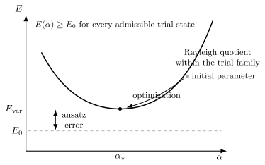
A parameterized trial family produces an energy landscape $E(\alpha)$. Optimization removes parameter error within that family, but the best value $E_{\mathrm{var}}$ can remain above $E_0$ because the exact ground state is not contained in the ansatz.

Where the Approximation Enters

The variational inequality itself is not approximate. Approximation enters when the full form domain is replaced by a tractable trial set $\mathcal T$. Define

$$E_{\mathcal T} = \inf_{ \substack{ \psi\in\mathcal T\\ \psi\ne0 } } \mathcal R_H[\psi].$$

Then

$$E_{\mathcal T} \geq E_0.$$

A numerical calculation usually adds two more layers. If $E_{\mathrm{opt}}$ is the best value actually found and $E_{\mathrm{rep}}$ is the reported, numerically evaluated value, then the error ledger is

$$\begin{aligned} E_{\mathrm{rep}}-E_0 ={}& \underbrace{E_{\mathcal T}-E_0}_{\text{trial-set error}} \,+ \underbrace{E_{\mathrm{opt}}-E_{\mathcal T}}_{\text{optimization error}} \\ &+ \underbrace{E_{\mathrm{rep}}-E_{\mathrm{opt}}}_{\text{evaluation error}}. \end{aligned}$$

The first two terms are nonnegative when the definitions are exact. The evaluation term need not be. Quadrature bias, stochastic error, basis-conditioning error, Hamiltonian truncation, or measurement noise can make a reported number fall below the true energy expectation. The upper-bound guarantee applies to the exact Rayleigh quotient of an admissible state for the stated Hamiltonian, not automatically to every number emitted by an optimizer.

Four objects that should not be conflated

Object	Meaning	Typical source of error
Hamiltonian $H$	The model whose spectrum is being bounded	Model or effective-theory error
Trial set $\mathcal T$	States the calculation is allowed to explore	Ansatz or basis incompleteness
Objective evaluator	Procedure for computing $\mathcal R_H$	Quadrature, sampling, truncation, or noise
Optimizer	Procedure for searching $\mathcal T$	Local minima, flat directions, poor conditioning

A low variational energy for one Hamiltonian does not bound the ground-state energy of a different Hamiltonian. This matters when pseudopotentials, finite boxes, basis cutoffs, or effective interactions are introduced.

Trial Sets and Ansätze

An ansatz is a deliberately restricted representation of a state. Its design should encode as much exact structure as possible before optimization begins. The detailed craft belongs to Trial Wavefunctions; the main families are summarized here.

Nonlinear parameterized states

A finite set of parameters $\boldsymbol\alpha$ defines

$$\lvert\psi(\boldsymbol\alpha)\rangle, \qquad \boldsymbol\alpha\in\mathcal P.$$

Widths, screening constants, correlation lengths, orbital exponents, and circuit angles are common examples. The objective

$$E(\boldsymbol\alpha) = \mathcal R_H[ \psi(\boldsymbol\alpha) ]$$

is generally nonlinear and can have several stationary points. A stationary point is not necessarily the global minimum over the trial family.

Energy gradients, projected tangents, parameter metrics, Hessians, constraints, and optimizer diagnostics are developed in Variational Parameters.

Linear trial subspaces

Choose basis states $\lvert\phi_j\rangle$ and vary their coefficients:

$$\lvert\psi(c)\rangle = \sum_{j=1}^{N} c_j\lvert\phi_j\rangle.$$

With

$$H_{ij} = \langle\phi_i\rvert H\lvert\phi_j\rangle, \qquad S_{ij} = \langle\phi_i\vert\phi_j\rangle,$$

stationarity gives the generalized eigenvalue problem

$$Hc=ESc.$$

Solving this matrix problem exactly performs the energy minimization exactly inside the chosen span. Basis truncation remains the approximation. This is the Rayleigh–Ritz Method.

Mixed linear and nonlinear ansätze

Many high-accuracy calculations combine both structures:

$$\lvert\psi(\boldsymbol\alpha,c)\rangle = \sum_{j=1}^{N} c_j \lvert\phi_j(\boldsymbol\alpha)\rangle.$$

For fixed $\boldsymbol\alpha$, the coefficients $c$ can be found by generalized diagonalization. An outer nonlinear loop then changes orbital shapes, Gaussian exponents, or other basis parameters. Separating the exact inner linear solve from the nonlinear outer search often improves stability and interpretability.

Stochastic evaluation

In many-body configuration space, deterministic integration can be impossible. Variational Monte Carlo samples $\lvert\psi\rvert^2$ and estimates the energy from the local energy. It preserves the conceptual variational structure, but finite-sample uncertainty and sampling bias must be reported separately. See Variational Monte Carlo Preview.

Time-dependent trial manifolds

The Time-Dependent Variational Principle projects Schrödinger evolution onto a manifold of parameterized states. Its purpose is not generally to minimize the instantaneous energy. It chooses the tangent-space motion that best satisfies an action or residual condition. The word “variational” therefore refers to a broader stationarity principle than the static ground-state bound.

Admissibility Comes Before Optimization

A flexible ansatz can still be invalid. Before evaluating an energy, check that each trial state has the properties required by the physical problem.

Normalizability and finite energy

A wavefunction may be square-integrable while its kinetic energy diverges. A cusp, discontinuity, or slowly decaying tail must be assessed using the quadratic form, not normalization alone.

For a one-dimensional kinetic term,

$$T = -\frac{\hbar^2}{2m} \frac{d^2}{dx^2},$$

the form expectation is often written

$$\langle T\rangle = \frac{\hbar^2}{2m} \int dx\, \left\lvert \frac{d\psi}{dx} \right\rvert^2,$$

after boundary terms have been shown to vanish. This expression makes the finite-gradient requirement visible.

Boundary conditions

Trial functions must respect hard walls, periodicity, self-adjoint boundary conditions, and regularity at singular points. Violating a boundary condition can enlarge the trial set beyond the Hamiltonian’s domain and destroy the claimed bound.

Exchange symmetry

For identical particles, the trial state must lie in the correct bosonic or fermionic sector. Antisymmetry is structural, not a small correction. Slater determinants enforce it for fermions, while correlation factors can be multiplied into an antisymmetric reference without changing particle-exchange parity.

Conserved symmetry sectors

Suppose $H$ preserves a sector $\mathcal H_q$, such as fixed parity or angular momentum. Minimization within that sector gives

$$E_{0}^{(q)} = \inf_{ \substack{ \psi\in\mathcal H_q\\ \psi\ne0 } } \mathcal R_H[\psi].$$

An admissible trial state in $\mathcal H_q$ satisfies

$$\mathcal R_H[\psi] \geq E_0^{(q)}.$$

The sector ground state may be an excited state of the full Hamiltonian. Symmetry adaptation can therefore target selected excitations while retaining a variational bound, provided the sector is truly invariant.

Choosing Parameters by Scale Analysis

Optimization works better when parameters reflect physical scales. Consider a schematic one-dimensional Hamiltonian

$$H = \frac{P^2}{2m} + g\lvert X\rvert^k, \qquad g\gt0, \quad k\gt0.$$

For a normalized trial family of width $b$, dimensional reasoning gives

$$\langle T\rangle \sim \frac{\hbar^2}{m b^2}, \qquad \langle V\rangle \sim g b^k.$$

Balancing the two terms predicts

$$b_\star \sim \left( \frac{\hbar^2}{mg} \right)^{1/(k+2)}$$

and the energy scale

$$E_\star \sim \left( \frac{\hbar^2}{m} \right)^{k/(k+2)} g^{2/(k+2)}.$$

The omitted numerical factors depend on the trial shape. Even so, scale analysis supplies sensible initial parameters, exposes unit mistakes, and suggests dimensionless optimization variables. A parameter search across many orders of magnitude is usually better performed in $\log b$ than in $b$ itself.

Upper Bounds and Systematic Improvement

If two trial sets are nested,

$$\mathcal T_1 \subseteq \mathcal T_2,$$

then

$$E_0 \leq E_{\mathcal T_2} \leq E_{\mathcal T_1}.$$

Enlarging the allowed set cannot worsen the exact optimized energy because every old trial state remains available. This monotonicity is one of the strongest diagnostics in basis-set calculations.

The statement needs all of its qualifiers:

• the Hamiltonian and its matrix elements must be unchanged;
• the trial sets must actually be nested;
• each minimization must be sufficiently converged;
• numerical evaluation must be accurate enough to resolve the difference.

Changing a nonlinear ansatz from one family to another does not generally produce a monotone sequence. Neither family may contain the other.

A bound is not an error bar

From

$$E_{\mathrm{var}} \geq E_0$$

alone, one cannot infer the size of $E_{\mathrm{var}}-E_0$. A certified lower bound, an exact comparison value, a converged numerical benchmark, or an additional theorem is needed to bracket the error. Agreement between two upper bounds is evidence, not a proof, because two ansätze can share the same bias.

Excited states and the min–max principle

The ground-state inequality does not by itself make an arbitrary excited-state ansatz an upper bound to a chosen excited level. For discrete eigenvalues ordered as $E_0\leq E_1\leq\cdots$, the relevant statement is the min–max characterization

$$E_k = \inf_{ \substack{ \mathcal S\subset\mathcal H\\ \dim\mathcal S=k+1 } } \; \sup_{ \substack{ \psi\in\mathcal S\\ \psi\ne0 } } \mathcal R_H[\psi].$$

Ritz eigenvalues inherit upper-bound properties under the theorem’s hypotheses. By contrast, minimizing over states orthogonal to inaccurate approximations of lower eigenstates does not automatically produce a rigorous bound to the next exact level. Upper Bounds and the Min–Max Principle gives the theorem, proof, essential-spectrum caveats, and interlacing results; the Rayleigh–Ritz Method develops the matrix construction.

Energy Accuracy and State Accuracy

The variational energy is often more accurate than the trial state. This useful property can become a trap if energy agreement is treated as a universal validation.

Assume a nondegenerate ground state and a positive spectral gap

$$\Delta = E_1-E_0 \gt0.$$

For a normalized trial state,

$$\begin{aligned} E[\psi]-E_0 ={}& \sum_{n\gt0} \lvert c_n\rvert^2(E_n-E_0) \\ \geq{}& \Delta \sum_{n\gt0} \lvert c_n\rvert^2. \end{aligned}$$

Therefore

$$1- \lvert\langle0\vert\psi\rangle\rvert^2 \leq \frac{E[\psi]-E_0}{\Delta}.$$

This converts an energy error into a fidelity guarantee only when $E_0$ and a usable gap bound are known. If $\Delta$ is small, a tiny energy error can coexist with substantial mixing. For a degenerate ground space, replace the overlap with $\langle\psi\rvert P_0\lvert\psi\rangle$, where $P_0$ projects onto that space.

For a bounded observable $A$, the pure-state trace-distance inequality gives

$$\left\lvert \langle A\rangle_\psi - \langle A\rangle_0 \right\rvert \leq 2\lVert A\rVert \sqrt{ 1- \lvert\langle0\vert\psi\rangle\rvert^2 }.$$

Combining the two bounds yields

$$\left\lvert \langle A\rangle_\psi - \langle A\rangle_0 \right\rvert \leq 2\lVert A\rVert \sqrt{ \frac{E[\psi]-E_0}{\Delta} }.$$

No corresponding conclusion follows for an arbitrary unbounded observable without extra assumptions. Short-distance densities, high moments, cusp-sensitive quantities, and tails can converge much more slowly than the energy.

A Two-Level Diagnostic Model

Let

$$\begin{aligned} H ={}& E_0\lvert0\rangle\langle0\rvert + E_1\lvert1\rangle\langle1\rvert, \\ \Delta ={}& E_1-E_0 \gt0, \end{aligned}$$

and consider

$$\lvert\psi(\theta,\phi)\rangle = \cos\theta\lvert0\rangle + e^{i\phi} \sin\theta\lvert1\rangle.$$

The energy landscape is

$$E(\theta) = E_0 + \Delta\sin^2\theta.$$

Several general lessons are visible in this small model:

1. The minimum occurs at the exact ground state, modulo phase and periodic parameter redundancy.
2. The energy error is quadratic in the small state-amplitude error $\sin\theta$.
3. The energy is independent of $\phi$, although observables with off-diagonal matrix elements can depend on $\phi$.
4. A small gap makes the landscape shallow and parameter estimation ill-conditioned.

The energy variance is

$$\begin{aligned} \sigma_H^2 ={}& \langle H^2\rangle - \langle H\rangle^2 \\ ={}& \Delta^2 \sin^2\theta \cos^2\theta. \end{aligned}$$

It vanishes at both exact eigenstates. Variance can diagnose whether a state is close to some eigenstate, but energy or symmetry information is needed to identify which one.

Diagnostics Beyond the Energy

A mature variational calculation reports how the result was challenged. No single diagnostic is sufficient in every problem.

Nested-space convergence

Increase a basis cutoff or enlarge a genuinely nested trial space. The optimized energy should decrease toward a stable value. Nonmonotonic behavior signals incomplete optimization, numerical error, or non-nested approximations.

Residual and energy variance

For a normalized trial state with energy $E=\langle H\rangle$, define

$$\lvert r\rangle = (H-E)\lvert\psi\rangle.$$

When $\psi$ lies in the operator domain of $H$,

$$\lVert r\rVert^2 = \langle(H-E)^2\rangle = \sigma_H^2.$$

An exact eigenstate has zero residual. A small residual is stronger evidence of local eigen-equation accuracy than a low energy alone, although interpreting it quantitatively still requires spectral information.

In a projected Rayleigh–Ritz calculation, the residual is orthogonal to the trial subspace at a stationary Ritz vector:

$$\langle\phi_j\vert r\rangle = 0, \qquad j=1,\ldots,N.$$

This Galerkin orthogonality does not imply $r=0$ outside the subspace.

Symmetry and exact identities

Check conserved quantum numbers, exchange symmetry, parity, and known commutator identities. The Hellmann–Feynman Theorem and virial relations can supply useful diagnostics, but only when their assumptions and parameter dependence are handled correctly.

Independent trial families

Compare ansätze with different structural biases: Gaussian versus exponential tails, coordinate-space versus basis-space representations, or deterministic versus stochastic evaluation. Agreement is more informative when the approximations fail differently.

Observable convergence

Track the observables relevant to the scientific question, not just the optimized objective. Energy convergence does not guarantee convergence of radii, contact densities, transition matrix elements, entanglement, or response functions.

Numerical conditioning

In a nonorthogonal basis, inspect the spectrum or condition number of the overlap matrix $S$. Near-linear dependence can produce apparently dramatic energy improvements that are numerical artifacts. Removing redundant directions or using a rank-revealing orthogonalization is part of the method, not housekeeping.

Method Roadmap

Question	Natural formulation	Continue with
Why is the ground-state estimate an upper bound?	Rayleigh quotient over the energy form domain	Variational Principle
How should physical information enter an ansatz?	Boundary, symmetry, scale, cusp, and tail constraints	Trial Wavefunctions
How are nonlinear ansatz coordinates optimized and diagnosed?	Gradients, tangent metrics, Hessians, and constrained searches	Variational Parameters
What does a complete one-parameter calculation look like?	Gaussian width for a problem with a known exact answer	Variational Estimate for the Harmonic Oscillator
How do Gaussian widths generalize to coupled coordinates?	Positive-definite width matrices and correlated Gaussian bases	Gaussian Variational Methods
How can a divergent weak-coupling series be reorganized around an adjustable reference problem?	Formal δ interpolation, order-dependent re-expansion, and optimization	Variational Perturbation Theory
How is a linear trial space optimized?	Hamiltonian and overlap matrices	Rayleigh–Ritz Method
Which excited-state Ritz values remain rigorous upper bounds?	Ordered subspace optimization below essential spectrum	Upper Bounds and the Min–Max Principle
How does screening improve a two-electron estimate?	Effective-charge product state	Variational Estimate for the Helium Atom
How can a parameterized state follow real-time motion?	Tangent-space projection or action stationarity	Time-Dependent Variational Principle
How are high-dimensional expectations evaluated stochastically?	Sampling $\lvert\psi\rvert^2$ and local energy	Variational Monte Carlo Preview
How should a suspicious result be diagnosed?	Symptom, failed assumption, quantitative test, and repair	Common Variational Pitfalls

Connections to Other Approximation Strategies

Perturbation theory

Perturbation theory expands around a solved Hamiltonian and can deliver analytic corrections order by order. A truncated perturbation series is not generally an upper bound. Variational methods instead optimize over states and can remain useful when no small coupling is available, but their accuracy depends strongly on ansatz design. The two approaches can be combined by using perturbative insight to construct or improve a trial family. Variational Perturbation Theory develops a more systematic hybrid in which an adjustable reference Hamiltonian is introduced, the series is re-expanded, and the residual parameter dependence is optimized at each order.

Semiclassical methods

WKB and related methods organize an asymptotic expansion in a scale ratio such as the de Broglie wavelength divided by a potential-variation length. Their errors have a different character from variational ansatz bias. Comparing a variational upper bound with a semiclassical estimate can be informative, but the semiclassical value does not automatically provide a lower bound.

Many-body and electronic-structure methods

Hartree–Fock, configuration interaction, matrix-product states, tensor-network methods, and many neural-network quantum states are variational when they minimize the expectation value of a specified Hamiltonian over a restricted state class. Each changes the expressive family and the optimization problem; none removes the need to separate model, ansatz, evaluation, and optimization errors.

Variational quantum eigensolvers

A variational quantum eigensolver prepares a parameterized state and estimates Hamiltonian expectation values. In the ideal mathematical description, the exact expectation of the prepared state obeys the same upper bound. Finite measurement statistics, device noise, imperfect Hamiltonian decomposition, and error mitigation can make the reported estimator nonvariational. The word “variational” should not be used as a substitute for an uncertainty budget.

Common Failure Modes

• Using an inadmissible state. Normalization alone does not establish finite energy or correct boundary conditions.
• Treating an upper bound as a symmetric error bar. The variational principle controls the sign, not the magnitude, of the energy error.
• Optimizing a modified objective. Penalty terms, truncated Hamiltonians, or noisy estimators may not bound the original Hamiltonian.
• Stopping at a stationary point. A zero gradient can identify a maximum, saddle, or local minimum.
• Comparing non-nested ansätze as though convergence must be monotone. Monotonicity follows from set inclusion, not from increasing a parameter count.
• Ignoring overlap-matrix conditioning. Nearly dependent basis vectors can corrupt generalized eigenvalues.
• Forgetting symmetry sectors. A low energy in the wrong sector does not approximate the targeted state.
• Using approximate orthogonality to claim an excited-state bound. Excited-state guarantees require the min–max structure or exact constraints.
• Equating energy accuracy with wavefunction accuracy. Small gaps and insensitive observables can hide substantial state error.
• Optimizing before checking scales. Poorly scaled parameters create flat directions and avoidable numerical instability.

The Common Variational Pitfalls guide turns these warnings into symptom-to-test-to-repair workflows, including boundary-domain failures, state-versus-energy accuracy, noisy estimators, and comparisons with perturbation theory.

Exercises

1. Scale invariance of the Rayleigh quotient

Show that $\mathcal R_H[c\psi]=\mathcal R_H[\psi]$ for every nonzero complex $c$. Explain why minimizing the unnormalized numerator alone is not an equivalent procedure.

Solution

The numerator and denominator transform as

$$\langle c\psi\rvert H\lvert c\psi\rangle = \lvert c\rvert^2 \langle\psi\rvert H\lvert\psi\rangle,$$ $$\langle c\psi\vert c\psi\rangle = \lvert c\rvert^2 \langle\psi\vert\psi\rangle.$$

The factors cancel in the quotient. By contrast, the unnormalized numerator can be driven toward zero by taking $c\to0$, regardless of the state’s shape. One must either constrain the norm or minimize the quotient.

2. Nested trial spaces

Let $\mathcal T_1\subseteq\mathcal T_2$. Prove that their exact optimized energies obey $E_{\mathcal T_2}\leq E_{\mathcal T_1}$. Does this prove that either value is close to $E_0$?

Solution

The infimum over $\mathcal T_2$ is taken over every state in $\mathcal T_1$ plus possibly more states. Therefore

$$\inf_{\psi\in\mathcal T_2} \mathcal R_H[\psi] \leq \inf_{\psi\in\mathcal T_1} \mathcal R_H[\psi].$$

Together with the variational principle,

$$E_0 \leq E_{\mathcal T_2} \leq E_{\mathcal T_1}.$$

This proves monotone improvement of the upper bound, not closeness to $E_0$. Both trial spaces can omit an important feature and remain far above the exact ground energy.

3. Two-level energy and variance

For the two-level trial state in the text, derive $E(\theta)$ and $\sigma_H^2$. Identify every value of $\theta$ for which the variance vanishes.

Solution

The occupation probabilities are $\cos^2\theta$ and $\sin^2\theta$, so

$$\begin{aligned} E(\theta) ={}& E_0\cos^2\theta + E_1\sin^2\theta \\ ={}& E_0+\Delta\sin^2\theta. \end{aligned}$$

Similarly,

$$\langle H^2\rangle = E_0^2\cos^2\theta + E_1^2\sin^2\theta.$$

Subtracting $E^2$ gives

$$\sigma_H^2 = \Delta^2 \sin^2\theta \cos^2\theta.$$

The variance vanishes when $\sin\theta=0$ or $\cos\theta=0$, corresponding to either exact energy eigenstate. Zero variance alone does not select the ground state.

4. Fidelity from an energy estimate

A normalized trial state has energy $E_0+\varepsilon$ for a Hamiltonian with a nondegenerate ground state and gap $\Delta\gt0$. Derive a lower bound on the ground-state fidelity. What does the bound say if $\varepsilon\geq\Delta$?

Solution

Writing $F=\lvert\langle0\vert\psi\rangle\rvert^2$, the gap inequality gives

$$\varepsilon \geq \Delta(1-F).$$

Hence

$$F \geq 1- \frac{\varepsilon}{\Delta}.$$

If $\varepsilon\geq\Delta$, the right side is nonpositive and the inequality supplies no nontrivial fidelity information. The variational energy remains an upper bound, but the gap estimate is then too weak to certify overlap.

5. A symmetry-sector bound

Suppose $[H,P]=0$ and $P^2=P=P^\dagger$. Let $\mathcal H_P$ be the range of $P$. Show that minimizing the Rayleigh quotient over $\mathcal H_P$ bounds the lowest energy in that invariant sector, even if that state is not the absolute ground state.

Solution

Because $[H,P]=0$, the range of $P$ is invariant under $H$. Restricting $H$ to $\mathcal H_P$ gives a self-adjoint sector Hamiltonian under the appropriate domain assumptions. Applying the variational principle to this restriction yields

$$\mathcal R_H[\psi] \geq E_0^{(P)}, \qquad \psi\in\mathcal H_P.$$

The value $E_0^{(P)}$ is the bottom of the spectrum in that sector. Another sector can contain a lower state, so $E_0^{(P)}$ need not equal the absolute ground energy.

6. Width scaling in a quartic trap

For $H=P^2/(2m)+gX^4$ with $g\gt0$, use scale balancing to determine the dependence of the optimal width and energy on $m$, $g$, and $\hbar$. Numerical constants are not required.

Solution

For a trial state of width $b$,

$$E(b) \sim \frac{\hbar^2}{m b^2} + g b^4.$$

Balancing the two contributions gives

$$\frac{\hbar^2}{m b^2} \sim g b^4,$$

so

$$b_\star \sim \left( \frac{\hbar^2}{mg} \right)^{1/6}.$$

Substitution gives

$$E_\star \sim \left( \frac{\hbar^2}{m} \right)^{2/3} g^{1/3}.$$

An explicit ansatz fixes the dimensionless prefactors but cannot change these scalings.

References

1. W. Ritz, “Über eine neue Methode zur Lösung gewisser Variationsprobleme der mathematischen Physik”, Journal für die reine und angewandte Mathematik 135, 1–61 (1909). The foundational finite-basis variational construction.
2. J. K. L. MacDonald, “Successive Approximations by the Rayleigh–Ritz Variation Method”, Physical Review 43, 830–833 (1933). A classic account of variational eigenvalue bounds and successive subspace approximations.
3. M. Reed and B. Simon, Methods of Modern Mathematical Physics, Vol. IV: Analysis of Operators (Academic Press, 1978), especially the spectral and min–max treatment. Bibliographic record.
4. R. K. Nesbet, Variational Principles and Methods in Theoretical Physics and Chemistry (Cambridge University Press, 2003). A graduate-level survey spanning bound states, time-dependent theory, and scattering applications.
5. E. A. Hylleraas, “Neue Berechnung der Energie des Heliums im Grundzustande, sowie des tiefsten Terms von Ortho-Helium”, Zeitschrift für Physik 54, 347–366 (1929). A landmark correlated variational calculation for helium.
6. R. McLachlan, “A variational solution of the time-dependent Schrödinger equation”, Molecular Physics 8, 39–44 (1964). A foundational residual-minimization formulation for variational dynamics.
7. W. M. C. Foulkes, L. Mitas, R. J. Needs, and G. Rajagopal, “Quantum Monte Carlo simulations of solids”, Reviews of Modern Physics 73, 33–83 (2001). A detailed review of variational and diffusion Monte Carlo, including optimization and statistical issues.