Time-Dependent Variational Principle

The time-dependent variational principle, or TDVP, replaces exact Schrödinger evolution by motion on a chosen manifold of trial states. At each instant, the exact velocity is compared with the velocities available inside that manifold, and a projection rule selects the parameter motion.

This is a dynamical approximation principle, not the Rayleigh–Ritz upper-bound principle. A TDVP trajectory need not provide an upper bound to a time-dependent observable, and a small energy expectation alone does not certify accurate dynamics.

Several related constructions are called “the TDVP.” The name can refer to:

• the Dirac–Frenkel condition, a complex orthogonality condition;
• the McLachlan principle, a least-squares projection in the real Hilbert-space metric;
• stationarity of the quantum action, which produces a symplectic flow.

They agree on important variational manifolds, especially complex or Kähler manifolds, but not on every real parameterization. Keeping that distinction visible prevents many apparent contradictions.

This page develops the common projection framework and its diagnostics. The geometry of rays itself is treated in Projective Hilbert Space, while exact Schrödinger evolution as Hamiltonian flow is developed in Hamiltonian Flow on Projective Hilbert Space.

The approximation problem

Let $H(t)$ be self-adjoint on a Hilbert space $\mathcal H$. Exact normalized states obey

$$i\hbar\lvert\dot\psi\rangle = H(t)\lvert\psi\rangle.$$

Choose instead a differentiable family of normalized trial states

$$\mathcal M = \left\{ \lvert\psi(\theta)\rangle: \theta=(\theta^1,\ldots,\theta^d)\in\Theta \right\},$$

where the coordinates $\theta^a$ are real unless stated otherwise. A path on $\mathcal M$ has velocity

$$\begin{aligned} \lvert\dot\psi\rangle &= \dot\theta^a\lvert\partial_a\psi\rangle, \\ \lvert\partial_a\psi\rangle &= \frac{\partial}{\partial\theta^a} \lvert\psi(\theta)\rangle. \end{aligned}$$

Repeated parameter indices are summed. The central difficulty is immediate: $-iH\lvert\psi\rangle/\hbar$ generally does not belong to the tangent space $T_\psi\mathcal M$. The variational ansatz can then reproduce only part of the exact velocity.

The quality of TDVP is therefore controlled by two separate choices:

1. Representation: does $\mathcal M$ contain states close to the exact trajectory?
2. Projection: how is the unavailable component of the exact velocity discarded?

The first is an approximation question; the second is a geometric one.

Rays, phase, and horizontal tangent vectors

A normalized state vector still contains an arbitrary phase. The vectors $\lvert\psi\rangle$ and $e^{i\alpha}\lvert\psi\rangle$ represent the same physical ray, so the direction $i\lvert\psi\rangle$ is a gauge direction rather than a physical deformation.

Introduce the projector orthogonal to the state,

$$Q_\psi = I-\lvert\psi\rangle\langle\psi\rvert,$$

and the horizontal tangent vectors

$$\lvert e_a\rangle = Q_\psi\lvert\partial_a\psi\rangle.$$

The physical tangent space represented by the chosen real coordinates is

$$T^{\mathrm{hor}}_\psi\mathcal M = \operatorname{span}_{\mathbb R} \{\lvert e_1\rangle,\ldots,\lvert e_d\rangle\}.$$

For a normalized state, the energy expectation is

$$E(\theta,t) = \langle\psi\rvert H(t)\lvert\psi\rangle.$$

Projecting Schrödinger’s equation with $Q_\psi$ removes the vertical phase velocity. The exact horizontal velocity is

$$\lvert v_H\rangle = -\frac{i}{\hbar} (H-E)\lvert\psi\rangle.$$

It is orthogonal to $\lvert\psi\rangle$. The variational problem is now cleanly stated: choose

$$\lvert\dot\psi_\perp\rangle = \dot\theta^a\lvert e_a\rangle$$

to approximate $\lvert v_H\rangle$ according to a specified projection principle.

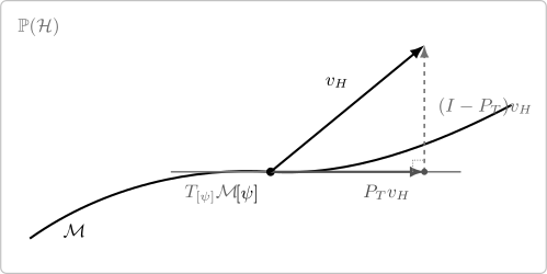
TDVP replaces the exact horizontal velocity $v_H$ by an allowed tangent velocity. For McLachlan projection, the discarded residual is orthogonal to the real tangent space in the Hilbert metric. Different variational principles use related but not always identical notions of projection.

If the trial state includes an explicit phase,

$$\lvert\Psi(t)\rangle = e^{i\phi(t)}\lvert\psi(\theta(t))\rangle,$$

then projection of Schrödinger’s equation along $\lvert\psi\rangle$ gives

$$\dot\phi = i\langle\psi\vert\dot\psi\rangle - \frac{E}{\hbar}.$$

In the horizontal gauge, $\langle\psi\vert\dot\psi\rangle=0$, so $\dot\phi=-E/\hbar$. Other gauges are equally valid, but the same convention must be used when comparing state-vector errors or residuals.

Metric and symplectic data

The projected tangent vectors define the quantum geometric tensor restricted to the variational manifold,

$$G_{ab} = \langle e_a\vert e_b\rangle.$$

Its real and imaginary parts supply two different geometric structures:

$$g_{ab} = \operatorname{Re}G_{ab}, \qquad \omega_{ab} = 2\hbar\operatorname{Im}G_{ab}.$$

Here $g_{ab}$ is the pullback of the Fubini–Study metric, up to the convention-dependent overall normalization. It measures distinguishable changes of the ray. The antisymmetric matrix $\omega_{ab}$ is the pullback of the projective symplectic form.

The metric is positive semidefinite:

$$u^a g_{ab}u^b = \left\| u^a\lvert e_a\rangle \right\|^2 \geq 0.$$

It is singular when some parameter combination changes only the gauge or does not change the state at all. The symplectic form can be singular for a different reason: a real variational manifold may fail to contain the conjugate direction needed to pair every coordinate.

These two matrices are not interchangeable. McLachlan dynamics is organized by $g$; action TDVP is organized by $\omega$.

Dirac–Frenkel principle

Define the horizontal Schrödinger residual

$$\lvert R_\perp\rangle = i\hbar\lvert\dot\psi_\perp\rangle - (H-E)\lvert\psi\rangle.$$

The Dirac–Frenkel condition is

$$\langle\delta\psi\vert R_\perp\rangle =0$$

for every allowed complex tangent variation $\lvert\delta\psi\rangle$. Equivalently, the residual is orthogonal in the complex Hilbert inner product to the chosen complex tangent space.

Suppose the manifold has local complex coordinates $z^j$ and a complex-linear horizontal tangent space spanned by $\lvert e_j\rangle$. Define

$$G_{\bar i j} = \langle e_i\vert e_j\rangle, \qquad h_{\bar i} = \langle e_i\rvert(H-E)\lvert\psi\rangle.$$

Then Dirac–Frenkel gives

$$i\hbar G_{\bar i j}\dot z^j = h_{\bar i}.$$

When $G_{\bar i j}$ is nonsingular, this is a first-order system for the complex parameters. If the exact horizontal velocity lies in the tangent space, the residual vanishes and the variational trajectory is locally exact.

Why complex linearity matters

For real coordinates, $T^{\mathrm{hor}}_\psi\mathcal M$ is initially only a real vector space. Multiplication of an allowed tangent vector by $i$ need not produce another allowed tangent vector. In that case, the complex equation

$$\langle e_a\vert R_\perp\rangle=0$$

can impose twice as many real conditions as there are real velocities $\dot\theta^a$. It may have no solution.

One must then either:

• enlarge the ansatz so that the tangent space is closed under multiplication by $i$;
• choose a real projection principle such as McLachlan’s;
• or use the action principle when the pulled-back symplectic structure is adequate.

Writing a formally invertible complex matrix does not repair a variational family that lacks the required physical directions.

McLachlan principle

McLachlan’s principle chooses the available velocity that minimizes the residual norm,

$$\dot\theta = \underset{u\in\mathbb R^d}{\operatorname{argmin}} \left\| u^a\lvert e_a\rangle - \lvert v_H\rangle \right\|^2.$$

Because the coefficients $u^a$ are real, stationarity gives real orthogonality conditions,

$$\operatorname{Re} \langle e_a\vert \dot\psi_\perp-v_H \rangle =0.$$

The resulting normal equations are

$$g_{ab}\dot\theta^b = \frac{1}{\hbar} \operatorname{Im} \langle e_a\rvert(H-E)\lvert\psi\rangle.$$

This is an ordinary real least-squares projection. It always has a minimizer in finite dimensions, although the minimizing parameter velocity need not be unique when $g$ is singular. All minimizers generate the same tangent state velocity if the null directions are purely redundant.

The minimized norm

$$\epsilon_{\mathrm{loc}} = \left\| \dot\psi_\perp-v_H \right\|$$

is a local-in-time measure of what the ansatz cannot follow. It has units of inverse time. Multiplying by $\hbar$ gives the norm of the horizontal Schrödinger residual.

Solving a singular metric system

The instruction “invert $g$” is unsafe near redundant or nearly redundant coordinates. A reliable implementation should instead:

1. identify exact gauge and parameter redundancies analytically where possible;
2. inspect the spectrum or singular values of $g$;
3. verify that the right-hand side is compatible with the range of $g$;
4. solve on the supported subspace, for example with a rank-revealing factorization or Moore–Penrose pseudoinverse;
5. report the cutoff or regularization used.

Adding $\lambda I$ to $g$ may stabilize a noisy calculation, but it changes the projected velocity. The regularization scale is therefore part of the approximation and should be tested, not hidden.

Stationary-action principle

For a normalized trial family, consider the real action

$$\mathcal S[\theta] = \int_{t_0}^{t_1}dt\,\mathcal L,$$

with

$$\mathcal L = \frac{i\hbar}{2} \left( \langle\psi\vert\dot\psi\rangle - \langle\dot\psi\vert\psi\rangle \right) -E(\theta,t).$$

The first term is the pullback of the Berry one-form. Varying the parameters with fixed endpoints gives

$$\omega_{ab}\dot\theta^b = -\partial_a E.$$

The sign follows from the convention

$$\omega_{ab} = 2\hbar \operatorname{Im} \langle e_a\vert e_b\rangle.$$

Changing the sign used to define the symplectic form changes the displayed Hamilton equation, not the physical trajectory.

This form makes the classical structure explicit: the energy expectation is a Hamiltonian function on the variational manifold. When $\omega$ is nondegenerate, the equations determine a Hamiltonian vector field. When $\omega$ is degenerate, there may be constraints, gauge directions, or no solution for a generic energy gradient.

For a time-independent Hamiltonian, action TDVP conserves the variational energy whenever the equations are well posed:

$$\frac{dE}{dt} = \partial_aE\,\dot\theta^a = -\omega_{ab}\dot\theta^a\dot\theta^b =0.$$

The last equality uses antisymmetry of $\omega_{ab}$. This is a structural conservation statement, not an assertion that the conserved variational energy equals the exact energy for an inaccurate initial state.

When the principles agree

Suppose the horizontal tangent space is closed under multiplication by $i$. It then carries a complex structure $J$ induced by

$$J\lvert u\rangle=i\lvert u\rangle.$$

On such a tangent space,

$$\omega(u,Jv) = 2\hbar\,g(u,v).$$

The real and imaginary parts of the complex Dirac–Frenkel condition are then related by $J$. Under the usual regularity assumptions, Dirac–Frenkel, McLachlan, and stationary-action TDVP select the same tangent velocity.

This situation occurs for many coherent-state, Gaussian, and tensor-network manifolds after gauge redundancies have been treated correctly. Geometrically, the favorable setting is a Kähler variational manifold.

On a generic real or non-Kähler manifold, the conclusions change:

• Dirac–Frenkel may be overdetermined.
• McLachlan still defines a least-squares tangent velocity.
• the pulled-back symplectic form may be singular.
• McLachlan and action trajectories can differ.

The phrase “the three principles are equivalent” therefore needs hypotheses. Complementary parameters, complex tangent closure, and nonsingular geometric structures are mathematical conditions, not notational details.

A one-parameter counterexample

Consider the real meridian of the qubit Bloch sphere,

$$\lvert\psi(\theta)\rangle = \cos\frac{\theta}{2}\lvert0\rangle + \sin\frac{\theta}{2}\lvert1\rangle,$$

with

$$H=\frac{\hbar\Omega}{2}\sigma_z.$$

The tangent vector is real,

$$\lvert e_\theta\rangle = \frac{1}{2} \left( -\sin\frac{\theta}{2}\lvert0\rangle + \cos\frac{\theta}{2}\lvert1\rangle \right),$$

and $g_{\theta\theta}=1/4$. Direct evaluation gives

$$\langle e_\theta\rvert(H-E)\lvert\psi\rangle = -\frac{\hbar\Omega}{4}\sin\theta,$$

which is real. McLachlan’s equation therefore gives $\dot\theta=0$: among the real-meridian velocities, zero is closest to the exact velocity, which points into a missing relative-phase direction.

By contrast, the formal Dirac–Frenkel equation would require

$$\frac{i\hbar}{4}\dot\theta = -\frac{\hbar\Omega}{4}\sin\theta,$$

which has no real solution for generic $\theta$. The one-dimensional symplectic form also vanishes identically, so action TDVP cannot generate the motion. Enlarging the ansatz to the full Bloch sphere restores the missing conjugate direction.

This example isolates the issue: the failure is in the variational manifold, not in Schrödinger’s equation.

Worked example: a fixed linear subspace

Let $\{\lvert\phi_j\rangle\}_{j=1}^n$ be linearly independent, time-independent basis vectors, not necessarily orthonormal, and set

$$\lvert\psi(t)\rangle = \sum_{j=1}^n c_j(t)\lvert\phi_j\rangle.$$

The residual orthogonality conditions against every basis vector give

$$i\hbar S\dot c = H_{\mathcal V}c,$$

where

$$S_{ij} = \langle\phi_i\vert\phi_j\rangle, \qquad (H_{\mathcal V})_{ij} = \langle\phi_i\vert H\lvert\phi_j\rangle.$$

This is simply Schrödinger evolution projected onto

$$\mathcal V = \operatorname{span}_{\mathbb C} \{\lvert\phi_1\rangle,\ldots,\lvert\phi_n\rangle\}.$$

Because $\mathcal V$ is a complex-linear space, the projection principles agree. If $S$ is positive definite and $H$ is time independent, the projected norm is conserved:

$$\frac{d}{dt}(c^\dagger Sc)=0.$$

The projected energy is also conserved:

$$\frac{d}{dt}(c^\dagger H_{\mathcal V}c)=0.$$

If $H\mathcal V\subseteq\mathcal V$, then the subspace is invariant and the evolution is exact for every initial state in $\mathcal V$. Otherwise, the residual is the component of $H\lvert\psi\rangle$ outside $\mathcal V$.

This example connects TDVP with Galerkin projection, basis-set truncation, configuration interaction, and spectral methods. If the basis itself moves in time, additional connection terms $\langle\phi_i\vert\dot\phi_j\rangle$ appear; omitting them breaks covariance under time-dependent basis changes.

Worked example: a thawed Gaussian

The static normalization and covariance structure are developed in Gaussian Variational Methods. For dynamics in one dimension, use the normalized ansatz

$$\begin{gathered} \psi(x;t) = \frac{e^{i\phi(t)}}{(2\pi\sigma^2)^{1/4}} \\ {}\times \exp\left[-\frac{(x-q)^2}{4\sigma^2}\right] \\ {}\times \exp\left[ \frac{i}{\hbar}p(x-q) + \frac{i}{2\hbar} \frac{\pi_\sigma}{\sigma}(x-q)^2 \right]. \end{gathered}$$

Here:

• $q=\langle x\rangle$ is the center;
• $p=\langle \hat p\rangle$ is the mean momentum;
• $\sigma^2=\langle(x-q)^2\rangle$ is the position variance;
• $\pi_\sigma$ is the momentum conjugate to the width;
• $\phi$ carries the overall phase.

For

$$H=\frac{\hat p^2}{2m}+V(\hat x),$$

the variational energy is

$$E = \frac{p^2}{2m} + \frac{\pi_\sigma^2}{2m} + \frac{\hbar^2}{8m\sigma^2} + \langle V\rangle_{q,\sigma},$$

with

$$\langle V\rangle_{q,\sigma} = \int_{-\infty}^{\infty} \frac{dx}{\sqrt{2\pi\sigma^2}} e^{-(x-q)^2/(2\sigma^2)}V(x).$$

Up to a total time derivative and the phase term, the Berry part of the action is

$$p\dot q+\pi_\sigma\dot\sigma.$$

The action equations are therefore canonical:

$$\dot q=\frac{p}{m}, \qquad \dot p=-\partial_q\langle V\rangle_{q,\sigma},$$

and

$$\dot\sigma=\frac{\pi_\sigma}{m}, \qquad \dot\pi_\sigma = \frac{\hbar^2}{4m\sigma^3} - \partial_\sigma\langle V\rangle_{q,\sigma}.$$

The center feels the potential averaged over the packet, while the width feels both the averaged potential and a repulsive quantum-pressure term proportional to $\hbar^2/\sigma^3$.

Harmonic oscillator

For

$$V(x)=\frac{1}{2}m\omega^2x^2,$$

the Gaussian average is

$$\langle V\rangle_{q,\sigma} = \frac{1}{2}m\omega^2(q^2+\sigma^2).$$

The center obeys the classical equation

$$\ddot q+\omega^2q=0,$$

and the width obeys the Ermakov equation

$$\ddot\sigma+\omega^2\sigma = \frac{\hbar^2}{4m^2\sigma^3}.$$

Its stationary solution is

$$\sigma_0 = \sqrt{\frac{\hbar}{2m\omega}},$$

the root-mean-square width of the oscillator ground state. The full Gaussian manifold is invariant under quadratic Hamiltonians, so these equations reproduce exact Gaussian evolution. This includes squeezed states, whose widths oscillate rather than remain fixed.

For a generic anharmonic potential, exact evolution generates skewness, kurtosis, interference, and possibly packet splitting. A single Gaussian cannot represent those features. The TDVP trajectory may remain smooth and energy-conserving while becoming physically inaccurate, which is why residual and ansatz-enlargement tests are essential. The free-particle limit is discussed in Gaussian Wave Packets.

Conservation laws and symmetries

Conservation properties depend on both the variational principle and the geometry of the ansatz.

Norm

If the manifold consists of normalized states and the evolution is expressed in horizontal tangent vectors, norm preservation is built in. For an unnormalized linear ansatz, the projected equations preserve the induced norm when the projected Hamiltonian is Hermitian with respect to the overlap matrix.

Energy

For time-independent $H$, action TDVP conserves $E(\theta)$. McLachlan TDVP on a generic real manifold does not automatically inherit this result. It does conserve energy when it is equivalent to the action or Dirac–Frenkel formulation under the required geometric hypotheses.

For explicitly time-dependent $H(t)$, even exact dynamics gives

$$\frac{d}{dt}\langle H\rangle = \left\langle\frac{\partial H}{\partial t}\right\rangle,$$

so energy conservation is not the appropriate diagnostic.

Other Noether charges

Suppose a unitary group acts on the Hilbert space and leaves both the Hamiltonian and the variational manifold invariant. If the associated infinitesimal symmetry directions belong to the tangent space and the action formulation is regular, the corresponding variational Noether charges are conserved.

Symmetry of $H$ alone is insufficient. An ansatz that is not closed under the symmetry can violate the charge even when the exact evolution preserves it. Conversely, building a symmetry sector directly into the ansatz may enforce the charge exactly while excluding physically relevant symmetry-breaking states.

Residuals and a posteriori error control

For a phase-fixed variational path $\lvert u(t)\rangle$, define the full residual

$$\lvert R(t)\rangle = i\hbar\lvert\dot u(t)\rangle - H(t)\lvert u(t)\rangle.$$

The residual answers a local question: how badly does the proposed path fail to satisfy Schrödinger’s equation? It vanishes if and only if the path is exact in the chosen phase convention.

Let $\lvert\psi(t)\rangle$ be the exact solution with the same initial state and phase. Unitarity and Duhamel’s formula give the a posteriori bound

$$\left\| \psi(t)-u(t) \right\| \leq \frac{1}{\hbar} \int_0^t ds\, \lVert R(s)\rVert.$$

This bound is rigorous under the usual domain assumptions for the self-adjoint Hamiltonian. It can be conservative, but it turns a residual history into a cumulative state-vector error certificate.

For physical rays, an arbitrary phase mismatch can make the Hilbert-space norm misleading. Either align phases before applying the bound or formulate the diagnostic with horizontal residuals and a projective distance. The distinction matters in long simulations, where an innocuous accumulated phase can dominate $\lVert\psi-u\rVert$.

Residual monitoring should be combined with:

• convergence under enlargement of the variational manifold;
• comparison with exact or independently converged evolution on benchmark systems;
• conservation-law drift appropriate to the chosen principle;
• time-step refinement, which separates integration error from variational error;
• observables sensitive to directions omitted by the ansatz.

A tiny numerical time-step does not cure a large projection residual. Conversely, a rich ansatz does not compensate for a poorly resolved time integrator.

Imaginary-time projection

Normalized imaginary-time evolution is

$$\hbar\lvert\partial_\tau\psi\rangle = -(H-E)\lvert\psi\rangle.$$

Unlike real-time Schrödinger evolution, this is a gradient-like flow that suppresses excited-state components. McLachlan projection onto a normalized real variational manifold gives

$$g_{ab}\frac{d\theta^b}{d\tau} = -\frac{1}{\hbar} \operatorname{Re} \langle e_a\rvert(H-E)\lvert\psi\rangle.$$

Because

$$\partial_aE = 2\operatorname{Re} \langle e_a\rvert(H-E)\lvert\psi\rangle,$$

the parameter equation becomes

$$g_{ab}\frac{d\theta^b}{d\tau} = -\frac{1}{2\hbar}\partial_aE.$$

Thus imaginary-time TDVP is natural-gradient descent in the metric induced by the state manifold. On the supported subspace of $g$,

$$\frac{dE}{d\tau} = -\frac{1}{2\hbar} (\partial_aE)(g^+)^{ab}(\partial_bE) \leq 0,$$

where $g^+$ is the Moore–Penrose pseudoinverse and compatibility with the metric range is understood.

Imaginary-time evolution does not turn an inadequate ansatz into an exact ground-state method. It converges, at best, to a stationary point of the energy restricted to the chosen manifold. The result should be checked with the static variational diagnostics in Variational Parameters.

Coherent-state and semiclassical bridge

Coherent-state manifolds often carry natural canonical coordinates. Restricting the quantum action to such a manifold produces Hamilton equations for expectation-value coordinates, with quantum corrections encoded in the variational energy and geometry.

For Hamiltonians no more than quadratic in canonical operators, the appropriate Gaussian or coherent-state family is invariant and the resulting motion is exact. For more general Hamiltonians, the same equations are semiclassical approximations whose accuracy depends on spreading, deformation, and interference.

The exact coherent-state construction, driven oscillator, and relation to phase-space dynamics are developed in Coherent-State Dynamics. Coherent-State Semiclassics Preview compares this one-manifold projection with thawed Gaussians, coherent-state boundary-value saddles, and initial-value representations. TDVP supplies the projection logic; it does not by itself establish a classical limit.

Tensor-network bridge

A matrix product state (MPS) of fixed bond dimension is a nonlinear variational manifold. MPS TDVP projects $-iH\lvert\Psi\rangle$ onto its tangent space, converting many-body Schrödinger evolution into equations for the tensors.

The geometry has practical consequences:

• a one-site, fixed-bond-dimension TDVP keeps the state on the same smooth manifold and can preserve norm and energy to integration accuracy;
• fixed bond dimension prevents the ansatz from representing unrestricted entanglement growth;
• two-site variants can enlarge the effective bond space and then truncate it;
• truncation introduces an additional error and can modify exact conservation properties;
• gauge fixing is required because many tensor parameterizations represent the same physical state.

The residual measures the component of the many-body evolution that the current tangent space cannot represent. Bond-dimension convergence and truncation diagnostics remain necessary even when energy is conserved. The role of entanglement and bond dimension is introduced in Entanglement in Many-Body Physics; detailed MPS integration algorithms belong to computational many-body methods.

Variational quantum-simulation bridge

For a parameterized quantum circuit

$$\lvert\psi(\theta)\rangle = U(\theta)\lvert\psi_0\rangle,$$

McLachlan projection again produces a metric linear system for $\dot\theta$. Matrix elements of $g_{ab}$ and the force vector can, in principle, be estimated from circuit measurements and combined with a classical linear solver.

Three cautions are fundamental:

1. A real circuit parameterization need not have a complex-linear tangent space, so formal equivalence among variational principles must be checked.
2. Removing or including the global-phase direction changes the equations unless the corresponding correction is handled consistently.
3. Finite-shot noise and hardware noise perturb both sides of an often ill-conditioned linear system; regularization bias can then be comparable to projection error.

The variational equation is only one layer of the algorithmic error budget. Expressivity, measurement cost, conditioning, numerical integration, and device noise must be assessed separately.

Practical workflow

A reproducible TDVP calculation should make the following choices explicit.

1. Define the manifold

State the normalized ansatz, parameter domain, and any coordinate singularities. Identify whether the tangent space is real, complex-linear, or Kähler.

2. Remove redundancies

Fix phase, tensor-network gauge, orbital gauge, or other parameter redundancies. Construct horizontal tangent vectors or an equivalent gauge-fixed basis.

3. Name the principle

Specify Dirac–Frenkel, McLachlan, or stationary action. Do not label a real-part normal equation “Dirac–Frenkel” without explaining the restriction that produced it.

4. Assemble geometric data

Compute $g$, $\omega$, or the complex Gram matrix required by the chosen principle. Check rank and conditioning along the trajectory.

5. Solve and integrate

Use a rank-aware linear solver. Choose a time integrator suited to the structure and stiffness of the reduced equations. Time-step error and projection error are distinct.

6. Validate

Monitor residual norms, conserved quantities, parameter-domain boundaries, and convergence under ansatz enlargement and time-step refinement.

Common mistakes

• Confusing static and dynamical variational principles. Rayleigh–Ritz gives spectral bounds under specific hypotheses; TDVP gives projected equations of motion.
• Leaving the phase direction untreated. The raw tangent Gram matrix can then be singular or the residual can be dominated by a physically irrelevant phase.
• Claiming universal equivalence. Dirac–Frenkel, McLachlan, and action TDVP agree only under geometric and regularity assumptions.
• Blindly inverting a metric matrix. Near-null directions amplify numerical noise and can generate enormous, physically meaningless parameter velocities.
• Using conservation as the only accuracy test. A restricted Hamiltonian flow can conserve its own energy while following the wrong trajectory.
• Ignoring moving-basis terms. Time-dependent orbitals or basis functions contribute connection terms to the coefficient equations.
• Conflating integration and variational error. Smaller time steps reduce discretization error, not the component of the exact velocity outside the tangent space.
• Overinterpreting smooth parameter motion. A single packet may evolve smoothly after the exact state has split into branches that the ansatz cannot represent.
• Regularizing without a sensitivity study. A metric cutoff or diagonal shift changes the dynamics and belongs in the reported method.

Exercises

1. Phase equation and horizontal velocity

Let $\lvert\Psi\rangle=e^{i\phi}\lvert\psi(\theta)\rangle$ with $\langle\psi\vert\psi\rangle=1$. Project Schrödinger’s equation first along $\lvert\psi\rangle$ and then with $Q_\psi$. Derive the phase equation and the exact horizontal velocity.

Solution

Differentiation gives

$$\lvert\dot\Psi\rangle = e^{i\phi} \left( i\dot\phi\lvert\psi\rangle + \lvert\dot\psi\rangle \right).$$

After canceling $e^{i\phi}$, Schrödinger’s equation is

$$-\hbar\dot\phi\lvert\psi\rangle + i\hbar\lvert\dot\psi\rangle = H\lvert\psi\rangle.$$

Taking the inner product with $\langle\psi\rvert$ yields

$$-\hbar\dot\phi + i\hbar\langle\psi\vert\dot\psi\rangle =E,$$

and hence

$$\dot\phi = i\langle\psi\vert\dot\psi\rangle -\frac{E}{\hbar}.$$

Applying $Q_\psi$ removes every term proportional to $\lvert\psi\rangle$:

$$i\hbar Q_\psi\lvert\dot\psi\rangle = Q_\psi H\lvert\psi\rangle = (H-E)\lvert\psi\rangle.$$

Therefore

$$\lvert v_H\rangle = Q_\psi\lvert\dot\psi\rangle = -\frac{i}{\hbar}(H-E)\lvert\psi\rangle.$$

2. Missing qubit direction

For the real-meridian qubit ansatz in the counterexample, verify $g_{\theta\theta}=1/4$ and show explicitly why McLachlan gives $\dot\theta=0$ for $H=\hbar\Omega\sigma_z/2$. What state-space direction is missing?

Solution

The tangent vector is orthogonal to the state, so it is already horizontal. Its squared norm is

$$\begin{aligned} g_{\theta\theta} &= \langle e_\theta\vert e_\theta\rangle \\ &= \frac{1}{4} \left( \sin^2\frac{\theta}{2} + \cos^2\frac{\theta}{2} \right) \\ &= \frac{1}{4}. \end{aligned}$$

The force matrix element is

$$\begin{aligned} \langle e_\theta\rvert(H-E)\lvert\psi\rangle &= \langle e_\theta\rvert H\lvert\psi\rangle \\ &= -\frac{\hbar\Omega}{4}\sin\theta, \end{aligned}$$

where the $E$ term drops out by orthogonality. This number is real, so the McLachlan force is its imaginary part divided by $\hbar$ and vanishes. Since $g_{\theta\theta}\neq0$, $\dot\theta=0$.

Evolution under $\sigma_z$ changes the relative phase between $\lvert0\rangle$ and $\lvert1\rangle$. The ansatz includes only real amplitudes and therefore lacks the azimuthal Bloch-sphere direction. Multiplying the tangent by $i$ produces precisely a direction outside the real tangent space.

3. Conservation in a nonorthogonal subspace

Starting from $i\hbar S\dot c=H_{\mathcal V}c$, with $S=S^\dagger\gt0$ and $H_{\mathcal V}=H_{\mathcal V}^\dagger$ time independent, prove conservation of $c^\dagger Sc$ and $c^\dagger H_{\mathcal V}c$.

Solution

The equation and its adjoint are

$$i\hbar S\dot c=H_{\mathcal V}c, \qquad -i\hbar\dot c^\dagger S=c^\dagger H_{\mathcal V}.$$

Therefore

$$\begin{aligned} \frac{d}{dt}(c^\dagger Sc) &= \dot c^\dagger Sc+c^\dagger S\dot c \\ &= \frac{i}{\hbar}c^\dagger H_{\mathcal V}c - \frac{i}{\hbar}c^\dagger H_{\mathcal V}c =0. \end{aligned}$$

For the energy, use $\dot c=-iS^{-1}H_{\mathcal V}c/\hbar$ and its adjoint:

$$\begin{aligned} \frac{d}{dt}(c^\dagger H_{\mathcal V}c) ={}& \dot c^\dagger H_{\mathcal V}c + c^\dagger H_{\mathcal V}\dot c \\ ={}& \frac{i}{\hbar} c^\dagger H_{\mathcal V}S^{-1}H_{\mathcal V}c \\ &- \frac{i}{\hbar} c^\dagger H_{\mathcal V}S^{-1}H_{\mathcal V}c =0. \end{aligned}$$

4. Gaussian width dynamics

For the harmonic potential, derive the Ermakov equation from the canonical Gaussian equations. Find the stationary width and verify that the corresponding zero-point contribution to the energy is $\hbar\omega/2$ when $q=p=\pi_\sigma=0$.

Solution

For the harmonic oscillator,

$$\partial_\sigma\langle V\rangle_{q,\sigma} = m\omega^2\sigma.$$

Using $\dot\sigma=\pi_\sigma/m$ gives

$$\ddot\sigma = \frac{\dot\pi_\sigma}{m} = \frac{\hbar^2}{4m^2\sigma^3} - \omega^2\sigma,$$

which is the stated Ermakov equation. A stationary width obeys

$$\omega^2\sigma_0 = \frac{\hbar^2}{4m^2\sigma_0^3},$$

so

$$\sigma_0^2=\frac{\hbar}{2m\omega}.$$

At the stationary point, the width-dependent energy is

$$\begin{aligned} E_\sigma &= \frac{\hbar^2}{8m\sigma_0^2} + \frac{1}{2}m\omega^2\sigma_0^2 \\ &= \frac{\hbar\omega}{4} + \frac{\hbar\omega}{4} \\ &= \frac{\hbar\omega}{2}. \end{aligned}$$

5. Imaginary time as natural-gradient descent

Assume $g$ is positive definite. Starting from

$$g_{ab}\theta^{\prime b} = -\frac{1}{2\hbar}\partial_aE,$$

prove that the variational energy cannot increase with imaginary time. When can equality hold?

Solution

Solving for the velocity gives

$$\theta^{\prime a} = -\frac{1}{2\hbar} (g^{-1})^{ab}\partial_bE.$$

Hence

$$\begin{aligned} \frac{dE}{d\tau} &= \partial_aE\,\theta^{\prime a} \\ &= -\frac{1}{2\hbar} (\partial_aE)(g^{-1})^{ab}(\partial_bE) \\ &\leq0. \end{aligned}$$

Positive definiteness makes the quadratic form nonnegative. Equality holds exactly when $\partial_aE=0$ for every variational direction. This means the state is stationary within the manifold, not necessarily an exact eigenstate of $H$.

6. Residual accumulation

Let exact and variational states have the same initial condition and satisfy

$$\begin{aligned} i\hbar\lvert\dot\psi\rangle &=H\lvert\psi\rangle, \\ i\hbar\lvert\dot u\rangle &=H\lvert u\rangle+\lvert R\rangle. \end{aligned}$$

Use the unitary propagator $U(t,s)$ to derive the residual error bound.

Solution

Set $\lvert e(t)\rangle=\lvert u(t)\rangle-\lvert\psi(t)\rangle$. Then

$$i\hbar\lvert\dot e\rangle = H\lvert e\rangle+\lvert R\rangle, \qquad \lvert e(0)\rangle=0.$$

Variation of constants gives

$$\lvert e(t)\rangle = -\frac{i}{\hbar} \int_0^t ds\, U(t,s)\lvert R(s)\rangle.$$

Because $U(t,s)$ is unitary,

$$\begin{aligned} \lVert e(t)\rVert &\leq \frac{1}{\hbar} \int_0^t ds\, \lVert U(t,s)R(s)\rVert \\ &= \frac{1}{\hbar} \int_0^t ds\, \lVert R(s)\rVert. \end{aligned}$$

The comparison assumes a common phase convention. A time-dependent global phase changes the state-vector residual even though it leaves the physical ray unchanged.

References

• P. A. M. Dirac, The Principles of Quantum Mechanics, 4th ed., Oxford University Press (1958), especially the action formulation of quantum dynamics.
• J. Frenkel, Wave Mechanics: Advanced General Theory, Oxford University Press (1934).
• A. D. McLachlan, “A variational solution of the time-dependent Schrödinger equation,” Molecular Physics 8, 39–44 (1964), doi:10.1080/00268976400100041.
• P. Kramer and M. Saraceno, Geometry of the Time-Dependent Variational Principle in Quantum Mechanics, Lecture Notes in Physics 140, Springer (1981), doi:10.1007/3-540-10579-4.
• J. Broeckhove, L. Lathouwers, E. Kesteloot, and P. Van Leuven, “On the equivalence of time-dependent variational principles,” Chemical Physics Letters 149, 547–550 (1988), doi:10.1016/0009-2614(88)80380-4.
• L. Hackl, T. Guaita, T. Shi, J. Haegeman, E. Demler, and J. I. Cirac, “Geometry of variational methods: dynamics of closed quantum systems,” SciPost Physics 9, 048 (2020), doi:10.21468/SciPostPhys.9.4.048.
• C. Lubich, “On variational approximations in quantum molecular dynamics,” Mathematics of Computation 74, 765–779 (2005), doi:10.1090/S0025-5718-04-01685-0.
• C. Lubich, From Quantum to Classical Molecular Dynamics: Reduced Models and Numerical Analysis, European Mathematical Society (2008), doi:10.4171/067.
• E. J. Heller, “Time-dependent approach to semiclassical dynamics,” Journal of Chemical Physics 62, 1544–1555 (1975), doi:10.1063/1.430620.
• J. Haegeman, C. Lubich, I. Oseledets, B. Vandereycken, and F. Verstraete, “Unifying time evolution and optimization with matrix product states,” Physical Review B 94, 165116 (2016), doi:10.1103/PhysRevB.94.165116.
• X. Yuan, S. Endo, Q. Zhao, Y. Li, and S. C. Benjamin, “Theory of variational quantum simulation,” Quantum 3, 191 (2019), doi:10.22331/q-2019-10-07-191.