Variational Estimate for the Harmonic Oscillator

The harmonic oscillator is an unusually transparent test of the variational method. Its exact ground state and energy are already known, so every step of a trial-state calculation can be checked: admissibility, normalization, expectation values, optimization, the upper bound, and the quality of the optimized state.

The calculation also succeeds in the strongest possible way. A one-parameter Gaussian family contains the exact ground state, and minimizing its width recovers both the oscillator length and the zero-point energy. That success is a property of this well-matched ansatz, not a general promise that a one-parameter variational calculation will be exact.

This page owns the worked variational calculation. The exact spectrum and Hermite-function eigenstates remain in Quantum Harmonic Oscillator, while the general upper-bound proof belongs to the Variational Principle.

Problem and Natural Scale

Consider a particle of mass $m$ in one dimension with

$$H = \frac{P^2}{2m} + \frac12m\omega^2X^2.$$

The parameters satisfy $m\gt0$ and $\omega\gt0$.

In the position representation,

$$P = -i\hbar\frac{d}{dx},$$

so the energy quadratic form is

$$\begin{aligned} q_H[\psi] ={}& \frac{\hbar^2}{2m} \int_{-\infty}^{\infty} \lvert\psi'(x)\rvert^2\,dx \\ &+ \frac12m\omega^2 \int_{-\infty}^{\infty} x^2\lvert\psi(x)\rvert^2\,dx. \end{aligned}$$

The competing terms identify a natural length,

$$\ell = \sqrt{ \frac{\hbar}{m\omega} }.$$

We will recover this scale by optimization rather than insert it into the trial state from the start.

Gaussian Trial State

Choose the normalized, real, even family

$$\psi_b(x) = \frac{1}{(\pi b^2)^{1/4}} \exp\left( -\frac{x^2}{2b^2} \right).$$

The width parameter is restricted to $b\gt0$.

The parameter $b$ controls the wavefunction width. It is not the position standard deviation. Since

$$\lvert\psi_b(x)\rvert^2 = \frac{1}{\sqrt{\pi}b} \exp\left( -\frac{x^2}{b^2} \right),$$

the variance will be $b^2/2$.

This family is admissible for every $b\gt0$: each state is square-integrable, smooth, even, and has finite kinetic and potential energy. The positivity restriction prevents a redundant sign convention and is naturally enforced by a logarithmic parameter such as $b=b_{\mathrm{ref}}e^\eta$.

The same family is often written using an inverse-square width,

$$\alpha = \frac{1}{b^2},$$

as

$$\psi_\alpha(x) = \left( \frac{\alpha}{\pi} \right)^{1/4} e^{-\alpha x^2/2}.$$

Both parameterizations describe exactly the same set of rays. Mixing their meanings is a common source of reciprocal-width errors.

Normalization and Moments

The required Gaussian integrals are

$$\int_{-\infty}^{\infty} e^{-x^2/b^2}\,dx = \sqrt{\pi}b,$$ $$\int_{-\infty}^{\infty} x^2e^{-x^2/b^2}\,dx = \frac{\sqrt{\pi}}{2}b^3,$$

and

$$\int_{-\infty}^{\infty} x^4e^{-x^2/b^2}\,dx = \frac{3\sqrt{\pi}}{4}b^5.$$

The first confirms

$$\int_{-\infty}^{\infty} \lvert\psi_b(x)\rvert^2\,dx = 1.$$

Parity gives

$$\langle X\rangle_b = 0,$$

and the second moment is

$$\langle X^2\rangle_b = \frac{b^2}{2}.$$

Thus

$$(\Delta X)_b = \frac{b}{\sqrt2}.$$

The fourth moment,

$$\langle X^4\rangle_b = \frac{3b^4}{4},$$

will later provide an energy-variance check.

Kinetic-Energy Expectation

Differentiate the trial state:

$$\psi_b'(x) = -\frac{x}{b^2}\psi_b(x),$$ $$\psi_b''(x) = \left( \frac{x^2}{b^4} - \frac{1}{b^2} \right) \psi_b(x).$$

Direct substitution gives

$$\begin{aligned} \langle T\rangle_b &= -\frac{\hbar^2}{2m} \int_{-\infty}^{\infty} \psi_b(x)\psi_b''(x)\,dx \\ &= -\frac{\hbar^2}{2m} \left( \frac{\langle X^2\rangle_b}{b^4} - \frac{1}{b^2} \right) \\ &= \frac{\hbar^2}{4mb^2}. \end{aligned}$$

Integration by parts supplies a useful check. The Gaussian and its derivative vanish at infinity, so

$$\langle T\rangle_b = \frac{\hbar^2}{2m} \int_{-\infty}^{\infty} \lvert\psi_b'(x)\rvert^2\,dx = \frac{\hbar^2}{4mb^2}.$$

This form makes positivity explicit. Narrowing the state increases its momentum gradients and makes the kinetic energy diverge as $b^{-2}$.

The corresponding momentum moments are

$$\langle P\rangle_b = 0, \qquad \langle P^2\rangle_b = \frac{\hbar^2}{2b^2},$$

and therefore

$$(\Delta P)_b = \frac{\hbar}{\sqrt2b}.$$

Every member of the family saturates

$$(\Delta X)_b(\Delta P)_b = \frac{\hbar}{2}.$$

Minimum uncertainty alone does not select the ground-state width; the Hamiltonian determines which minimum-uncertainty Gaussian has the lowest energy.

Potential-Energy Expectation

The quadratic potential requires only $\langle X^2\rangle_b$:

$$\begin{aligned} \langle V\rangle_b &= \frac12m\omega^2 \langle X^2\rangle_b \\ &= \frac{m\omega^2b^2}{4}. \end{aligned}$$

The potential term has the opposite width dependence from the kinetic term. A broad state reduces gradients but samples larger values of $x^2$.

Energy Functional

Adding the two contributions gives

$$E(b) = \langle\psi_b\rvert H\lvert\psi_b\rangle = \frac{\hbar^2}{4mb^2} + \frac{m\omega^2b^2}{4}.$$

The upper-bound theorem guarantees

$$E(b) \geq E_0$$

for every $b\gt0$, where $E_0$ is the true ground-state energy. It does not yet tell us which width gives the best bound.

Introduce the dimensionless width ratio

$$s = \frac{b}{\ell}.$$

Using $\ell^2=\hbar/(m\omega)$, the energy becomes

$$\varepsilon(s) \equiv \frac{E(b)}{\hbar\omega} = \frac{1}{4s^2} + \frac{s^2}{4}.$$

All dimensions have disappeared. The two terms are the kinetic and potential contributions in units of $\hbar\omega$.

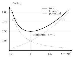
The kinetic contribution falls as $s^{-2}$ while the potential contribution rises as $s^2$. Their sum has its unique minimum at $s=b/\ell=1$, where the two contributions are equal and the Gaussian coincides with the exact ground state.

The limiting behavior is physically sensible:

Width regime	Kinetic energy	Potential energy	Total energy
$s\to0$	diverges	tends to zero	diverges
$s=1$	$\hbar\omega/4$	$\hbar\omega/4$	$\hbar\omega/2$
$s\to\infty$	tends to zero	diverges	diverges

Optimization

Differentiating with respect to the dimensional width gives

$$\frac{dE}{db} = -\frac{\hbar^2}{2mb^3} + \frac12m\omega^2b.$$

The stationary equation is

$$m\omega^2b = \frac{\hbar^2}{mb^3},$$

or

$$b^4 = \frac{\hbar^2}{m^2\omega^2} = \ell^4.$$

Because $b\gt0$, the only stationary width is

$$b_\star = \ell.$$

The second derivative is

$$\frac{d^2E}{db^2} = \frac{3\hbar^2}{2mb^4} + \frac12m\omega^2,$$

which is positive for every $b\gt0$. In particular,

$$\left. \frac{d^2E}{db^2} \right|_{b=\ell} = 2m\omega^2 \gt0.$$

The stationary point is therefore the unique global minimum. Substitution gives

$$E_{\mathrm{var}} = E(\ell) = \frac12\hbar\omega.$$

Optimization without calculus

The dimensionless expression can also be rearranged as

$$\begin{aligned} \varepsilon(s) &= \frac12 + \frac14 \left( s- \frac1s \right)^2 \\ &\geq \frac12. \end{aligned}$$

Equality holds only at $s=1$. This is the arithmetic–geometric-mean inequality in a form that displays the nonnegative energy excess.

Logarithmic width

For numerical work, write

$$s = e^\eta, \qquad \eta\in\mathbb R.$$

Then positivity is automatic and

$$\varepsilon(\eta) = \frac12\cosh(2\eta).$$

The optimum is $\eta_\star=0$. Near it,

$$\varepsilon(\eta) = \frac12 + \eta^2 + O(\eta^4).$$

The absence of a linear term is the local stationarity expected at a variational optimum. General parameter gradients, Hessians, and reparameterizations are developed in Variational Parameters.

Why the Bound Becomes Exact

At the optimum,

$$\psi_{b_\star}(x) = \frac{1}{(\pi\ell^2)^{1/4}} \exp\left( -\frac{x^2}{2\ell^2} \right),$$

which is the exact normalized oscillator ground state. The variational family happened to contain the target eigenvector.

This can be checked without importing the known spectrum. Acting with the Hamiltonian on a general family member gives the local-energy expression

$$\frac{H\psi_b(x)}{\psi_b(x)} = \frac{\hbar^2}{2mb^2} + \frac12 \left( m\omega^2 - \frac{\hbar^2}{mb^4} \right) x^2.$$

At $b=\ell$, the coefficient of $x^2$ vanishes and

$$H\psi_\ell = \frac12\hbar\omega\,\psi_\ell.$$

Thus the optimized state is not merely stationary inside the Gaussian family. It satisfies the full eigenvalue equation.

For $b\ne\ell$, the local energy depends on $x$, so the state is not an eigenstate. Its energy variance is

$$\begin{aligned} (\Delta H)_b^2 &= \langle H^2\rangle_b - E(b)^2 \\ &= \frac{(\hbar\omega)^2}{8} \left( s^2-s^{-2} \right)^2. \end{aligned}$$

It vanishes only at $s=1$. For a normalized state in the operator domain, this variance is also the squared residual norm,

$$(\Delta H)_b^2 = \left\lVert (H-E(b))\psi_b \right\rVert^2.$$

Energy minimization and residual vanishing therefore agree at the optimum in this example. In a restricted family that does not contain an eigenstate, the minimum energy generally has a nonzero residual outside the trial tangent space.

The Variational Monte Carlo Preview recasts this same local energy as a sampled estimator and explains how its variance controls both residual diagnostics and statistical uncertainty.

Exact Comparison and Error Measures

The exact ground-state energy is

$$E_0 = \frac12\hbar\omega,$$

so the variational excess at arbitrary width is

$$E(b)-E_0 = \frac{\hbar\omega}{4} \left( s- \frac1s \right)^2.$$

In the logarithmic coordinate,

$$\frac{E(b)-E_0}{\hbar\omega} = \sinh^2\eta.$$

The squared overlap with the exact ground state is

$$\begin{aligned} F(s) &= \left\lvert \langle\psi_\ell\vert\psi_b\rangle \right\rvert^2 \\ &= \frac{2s}{1+s^2} \\ &= \frac{1}{\cosh\eta}. \end{aligned}$$

Near the optimum,

$$1-F = \frac{\eta^2}{2} + O(\eta^4),$$

while

$$\frac{E-E_0}{\hbar\omega} = \eta^2 + O(\eta^4).$$

Both are second order here, but they quantify different objects. In more complicated variational families, a small energy error need not imply that every observable or wavefunction feature is comparably accurate.

Virial and Uncertainty Interpretations

At the stationary width,

$$\langle T\rangle_\star = \langle V\rangle_\star = \frac14\hbar\omega.$$

This is the harmonic-oscillator virial relation. In the present one-parameter family, changing $b$ is a scale transformation: the kinetic term scales as $b^{-2}$ and the quadratic potential as $b^2$. Stationarity under that scaling forces the two terms to balance.

Every trial Gaussian also saturates the position–momentum uncertainty relation. The optimizer chooses the member whose position and momentum spreads balance the coefficients in the Hamiltonian. The broader physical interpretation of this balance belongs to Zero-Point Energy.

A wrong-width centered Gaussian is a squeezed vacuum relative to the oscillator’s natural quadratures. With $s=e^\eta$, its energy is

$$E = \frac12\hbar\omega\cosh(2\eta).$$

The sign convention for the squeezing parameter may reverse $\eta$, but the energy is unchanged. The state interpretation is developed in Squeezed States: First Encounter.

Adding Center and Mean Momentum

The centered real ansatz already respects the parity and time-reversal properties of the nondegenerate ground state. To see what those choices save, enlarge the family to

$$\begin{aligned} \psi_{b,x_c,p_c}(x) ={}& \frac{1}{(\pi b^2)^{1/4}} \\ &\times \exp\left[ -\frac{(x-x_c)^2}{2b^2} \right] \\ &\times \exp\left[ \frac{i p_c(x-x_c)}{\hbar} \right]. \end{aligned}$$

Its moments are

$$\langle X\rangle = x_c, \qquad \langle P\rangle = p_c,$$ $$\langle X^2\rangle = x_c^2 + \frac{b^2}{2},$$

and

$$\langle P^2\rangle = p_c^2 + \frac{\hbar^2}{2b^2}.$$

Therefore

$$\begin{aligned} E(b,x_c,p_c) ={}& \frac{\hbar^2}{4mb^2} + \frac{m\omega^2b^2}{4} \\ &+ \frac{p_c^2}{2m} + \frac12m\omega^2x_c^2. \end{aligned}$$

Every added term is nonnegative. The optimizer returns

$$x_{c,\star} = 0, \qquad p_{c,\star} = 0, \qquad b_\star = \ell.$$

Building exact symmetries into the ansatz removed two parameters whose optimum was known in advance. Displacements and phase-space motion become useful for different targets, such as coherent states and displaced oscillators, but they do not improve this ground-state calculation.

A Deliberately Imperfect Trial Family

Exact recovery can hide the distinction between the theorem and the ansatz. Consider instead the normalized exponential

$$\chi_a(x) = \frac{1}{\sqrt a} e^{-\lvert x\rvert/a}, \qquad a\gt0.$$

This state has the correct even parity and is in the Hamiltonian’s quadratic-form domain, but its cusp and exponential tail do not match the smooth Gaussian oscillator ground state.

Using the form expression for kinetic energy,

$$\int_{-\infty}^{\infty} \lvert\chi_a'(x)\rvert^2\,dx = \frac{1}{a^2},$$

and

$$\langle X^2\rangle_\chi = \frac{a^2}{2}.$$

Its variational energy is

$$E_\chi(a) = \frac{\hbar^2}{2ma^2} + \frac{m\omega^2a^2}{4}.$$

For $t=a/\ell$,

$$\frac{E_\chi(t)}{\hbar\omega} = \frac{1}{2t^2} + \frac{t^2}{4}.$$

Stationarity gives

$$t_\star^4 = 2, \qquad t_\star = 2^{1/4},$$

and hence

$$E_{\chi,\star} = \frac{\hbar\omega}{\sqrt2} \gt \frac12\hbar\omega.$$

This is a valid but non-exact upper bound. The optimizer has found the best state in the exponential family; it cannot remove the family’s structural mismatch.

The cusp also illustrates why the form domain matters. A naive second derivative of $e^{-\lvert x\rvert/a}$ misses a delta distribution at the origin. The positive quadratic-form expression using the weak first derivative gives the correct variational kinetic energy without pretending that $\chi_a$ lies in the strong operator domain.

Lessons for Ansatz Design

1. Use natural scales without hard-coding the answer. The Hamiltonian suggests a competition between localization and spreading; optimization recovers $\ell$.
2. Respect exact symmetry. A real even ansatz is sufficient for the nondegenerate centered ground state.
3. Track conventions. The wavefunction width $b$, probability standard deviation $b/\sqrt2$, and inverse width $\alpha=1/b^2$ are different quantities.
4. Nondimensionalize early. The single ratio $s=b/\ell$ exposes the universal optimization problem.
5. Separate optimization error from ansatz error. The Gaussian optimum has neither; the exponential optimum retains ansatz error.
6. Check more than stationarity. Boundary behavior, second derivatives, limiting cases, residuals, and comparison with known results all test the calculation.
7. Do not generalize accidental exactness. A family gives the exact energy only when it contains a ground-state vector or another equality condition is met.

The same Gaussian width calculation becomes nontrivial after adding an anharmonic term. The quartic example in Variational Parameters shows how the optimum shifts when the exact ground state is no longer Gaussian. Gaussian Variational Methods generalizes the ansatz to coupled coordinates, positive-definite width matrices, and correlated Gaussian bases.

Common Mistakes

• Calling $b$ the standard deviation instead of $b/\sqrt2$.
• Forgetting that the normalization factor depends on the variational width.
• Dropping the minus sign in $P^2=-\hbar^2d^2/dx^2$.
• Missing the factor of $1/2$ in $\langle X^2\rangle=b^2/2$.
• Minimizing kinetic or potential energy separately instead of their sum.
• Keeping the unphysical negative solution of $b^4=\ell^4$ even though $b\gt0$.
• Concluding that every minimum-uncertainty Gaussian is an oscillator ground state.
• Treating a stationary point as sufficient without checking curvature or global limits.
• Claiming that the variational method is generally exact because this family contains the exact answer.
• Applying the strong second-derivative formula to a cusp without accounting for distributions or using the quadratic form.

Exercises

1. Reparameterize by inverse width

Set $\alpha=1/b^2$ and derive the energy $E(\alpha)$. Find the minimizing $\alpha$ and verify that it corresponds to $b=\ell$.

Solution

Substituting $b^2=1/\alpha$ gives

$$E(\alpha) = \frac{\hbar^2\alpha}{4m} + \frac{m\omega^2}{4\alpha}, \qquad \alpha\gt0.$$

The derivative is

$$\frac{dE}{d\alpha} = \frac{\hbar^2}{4m} - \frac{m\omega^2}{4\alpha^2}.$$

Stationarity requires

$$\alpha_\star^2 = \frac{m^2\omega^2}{\hbar^2}.$$

The positive solution is

$$\alpha_\star = \frac{m\omega}{\hbar} = \frac{1}{\ell^2}.$$

Therefore $b_\star=1/\sqrt{\alpha_\star}=\ell$ and $E(\alpha_\star)=\hbar\omega/2$.

2. Prove the global bound algebraically

Starting from

$$\varepsilon(s) = \frac{1}{4s^2} + \frac{s^2}{4},$$

show without differentiation that $\varepsilon(s)\geq1/2$ for every $s\gt0$. Determine the equality condition.

Solution

Complete a square:

$$\begin{aligned} \varepsilon(s)-\frac12 &= \frac14 \left( s^2+s^{-2}-2 \right) \\ &= \frac14 \left( s-s^{-1} \right)^2 \\ &\geq 0. \end{aligned}$$

Equality requires $s=s^{-1}$. Since $s\gt0$, this gives $s=1$.

3. Derive the displaced-packet energy

For $\psi_{b,x_c,p_c}$ in the text, compute $\langle X^2\rangle$ and $\langle P^2\rangle$, then derive the full energy functional and its minimum.

Solution

Writing $y=x-x_c$, the probability density is an even Gaussian in $y$. Hence

$$\langle X\rangle = x_c, \qquad \langle (X-x_c)^2\rangle = \frac{b^2}{2},$$

so

$$\langle X^2\rangle = x_c^2 + \frac{b^2}{2}.$$

The phase shifts the momentum mean by $p_c$ without changing its variance:

$$\langle P^2\rangle = p_c^2 + \frac{\hbar^2}{2b^2}.$$

Therefore

$$E = \frac{\hbar^2}{4mb^2} + \frac{m\omega^2b^2}{4} + \frac{p_c^2}{2m} + \frac12m\omega^2x_c^2.$$

The last two terms are minimized at $p_c=x_c=0$, and the width terms are minimized at $b=\ell$. The global minimum is $\hbar\omega/2$.

4. Check the energy variance

Use the local energy and the Gaussian moments to derive

$$(\Delta H)_b^2 = \frac{(\hbar\omega)^2}{8} \left( s^2-s^{-2} \right)^2.$$

Why does its vanishing give stronger information than $dE/db=0$?

Solution

Write the local energy as

$$E_L(x) = A+Bx^2,$$

where

$$\begin{aligned} A &= \frac{\hbar^2}{2mb^2}, \\ B &= \frac12 \left( m\omega^2 - \frac{\hbar^2}{mb^4} \right). \end{aligned}$$

Only the $Bx^2$ term fluctuates. Since

$$\operatorname{Var}(X^2) = \langle X^4\rangle - \langle X^2\rangle^2 = \frac{b^4}{2},$$

we obtain

$$(\Delta H)_b^2 = B^2\frac{b^4}{2}.$$

Substituting $b=s\ell$ and $\ell^2=\hbar/(m\omega)$ yields the stated expression. It vanishes only when $s=1$.

The condition $dE/db=0$ means that the residual is orthogonal to the single tangent direction generated by changing $b$. Zero variance means the full residual vanishes, so the state is an exact eigenstate.

5. Optimize the exponential trial state

Verify the normalization and moments of $\chi_a(x)=a^{-1/2}e^{-\lvert x\rvert/a}$. Derive its optimized energy and compare it with the exact ground energy.

Solution

Normalization follows from

$$\frac{2}{a} \int_0^\infty e^{-2x/a}\,dx = 1.$$

For $x\ne0$,

$$\lvert\chi_a'(x)\rvert^2 = \frac{1}{a^2} \lvert\chi_a(x)\rvert^2,$$

so the form-domain kinetic energy is

$$\langle T\rangle = \frac{\hbar^2}{2ma^2}.$$

Also,

$$\langle X^2\rangle = \frac{2}{a} \int_0^\infty x^2e^{-2x/a}\,dx = \frac{a^2}{2}.$$

Thus

$$\frac{E_\chi}{\hbar\omega} = \frac{1}{2t^2} + \frac{t^2}{4}, \qquad t = \frac{a}{\ell}.$$

The stationary equation is

$$-\frac{1}{t^3} + \frac{t}{2} = 0,$$

so $t_\star=2^{1/4}$. Substitution gives

$$E_{\chi,\star} = \frac{\hbar\omega}{\sqrt2}.$$

This exceeds the exact value $\hbar\omega/2$, as the variational theorem requires. The excess is caused by ansatz mismatch, not incomplete optimization.

6. Extend to an isotropic oscillator in d dimensions

For

$$H = \sum_{j=1}^{d} \left( \frac{P_j^2}{2m} + \frac12m\omega^2X_j^2 \right),$$

use the product Gaussian

$$\Psi_b(\mathbf x) = \prod_{j=1}^{d} \psi_b(x_j).$$

Find the optimized width and energy.

Solution

Each Cartesian factor contributes independently,

$$E_1(b) = \frac{\hbar^2}{4mb^2} + \frac{m\omega^2b^2}{4}.$$

Therefore

$$E_d(b) = dE_1(b).$$

Multiplication by the positive constant $d$ does not change the minimizing width, so

$$b_\star = \ell.$$

The optimized energy is

$$E_{d,\star} = \frac{d}{2}\hbar\omega.$$

The product family contains the exact isotropic-oscillator ground state, so the bound is saturated.

References

1. R. Shankar, Principles of Quantum Mechanics, 2nd ed. (Springer, 1994), chapters on the variational principle and harmonic oscillator.
2. D. J. Griffiths and D. F. Schroeter, Introduction to Quantum Mechanics, 3rd ed. (Cambridge University Press, 2018), for the oscillator and elementary variational estimates.
3. C. Cohen-Tannoudji, B. Diu, and F. Laloë, Quantum Mechanics, Vol. 1, 2nd ed. (Wiley-VCH, 2020), for Gaussian wave packets, the oscillator, and variational reasoning.
4. M. Reed and B. Simon, Methods of Modern Mathematical Physics, Vol. IV: Analysis of Operators (Academic Press, 1978), for the min–max principle and quadratic-form formulation. Bibliographic record.
5. W. Ritz, “Über eine neue Methode zur Lösung gewisser Variationsprobleme der mathematischen Physik”, Journal für die reine und angewandte Mathematik 135, 1–61 (1909), for the historical variational method.