Variational Perturbation Theory

Variational perturbation theory reorganizes a perturbative calculation around an adjustable solvable problem and fixes the auxiliary parameters only after truncation. The exact answer does not depend on those parameters. A finite-order approximation does, so its residual dependence can be reduced, inspected, and used as a diagnostic.

The method is valuable when ordinary perturbation theory is accurate only near a weak-coupling point, especially when its coefficients form a divergent asymptotic series. It can absorb part of the interaction into a better reference scale and can build known strong-coupling behavior into an order-dependent sequence. It is not a universal convergence machine, and the word variational does not mean that every optimized approximant is a rigorous upper bound.

This page is the canonical home for the interpolation, re-expansion, and order-by-order optimization procedure. The ordinary Rayleigh–Schrödinger recursion belongs to Higher-Order Structure, the quartic oscillator as a multi-method model belongs to Anharmonic Oscillator, and static Gaussian expectations and covariance formulas belong to Gaussian Variational Methods.

Why Reorganize a Perturbation Series?

Suppose an observable has a formal weak-coupling expansion

$$Q(g) \sim \sum_{n=0}^{\infty}a_n g^n.$$

Three different difficulties can arise.

1. The series can converge, but only inside a disk that does not reach the desired coupling.
2. The series can be asymptotic, so its terms eventually grow at every fixed $g\ne0$.
3. The first few terms can be poorly adapted to the physical scale of the interacting problem even before large-order growth becomes visible.

An adjustable reference Hamiltonian addresses the third problem directly and can sometimes address the first two. The guiding idea is simple: add and subtract a solvable term, treat the subtraction perturbatively, and let the reference scale depend on truncation order.

This changes the sequence of finite-order approximations without changing the exact problem. If every order could be summed, the auxiliary scale would disappear. At finite order, the scale records how the calculation was reorganized.

Core Construction

Let $H$ be the physical Hamiltonian. Choose a solvable family $H_0(\alpha)$ depending on one or more auxiliary parameters $\alpha$, and define

$$\Delta H(\alpha) = H-H_0(\alpha).$$

Introduce a bookkeeping parameter $\delta$:

$$H_\delta(\alpha) = H_0(\alpha) + \delta\Delta H(\alpha).$$

The endpoints are

$$H_{\delta=0}(\alpha)=H_0(\alpha), \qquad H_{\delta=1}(\alpha)=H.$$

For fixed $\alpha$, ordinary perturbation theory in $\delta$ gives

$$Q(\delta,\alpha) \sim \sum_{n=0}^{\infty} q_n(\alpha)\delta^n.$$

Truncate at order $N$ and only then set $\delta=1$:

$$Q_{[N]}(\alpha) = \left. \sum_{n=0}^{N} q_n(\alpha)\delta^n \right|_{\delta=1}.$$

The formal parameter $\delta$ is not normally a new physical coupling. It labels how far the interpolation has moved from the chosen reference problem to the physical one.

Exact auxiliary independence

At $\delta=1$, the exact Hamiltonian is $H$ for every admissible $\alpha$. An exact observable therefore satisfies

$$\frac{\partial Q}{\partial\alpha}=0.$$

The truncated expression generally does not:

$$\frac{\partial Q_{[N]}}{\partial\alpha} \ne0.$$

This residual dependence is a truncation artifact. Optimization attempts to choose a region where the artifact has the least local effect. It does not turn $\alpha$ into a measurable parameter.

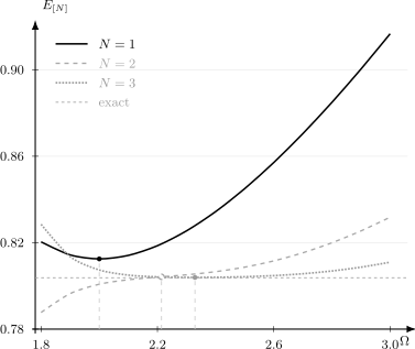
Residual auxiliary-frequency dependence at $g=1$ for the quartic-oscillator approximants derived below. Filled markers show the first- and third-order PMS points. The open marker is a second-order inflection point, used as a heuristic continuation because that curve has no real PMS point. The horizontal line is a converged numerical benchmark.

Optimization Prescriptions

The exact auxiliary independence does not specify a unique finite-order rule. Several prescriptions are used, and their equivalence must not be assumed.

Principle of minimal sensitivity

The principle of minimal sensitivity, or PMS, chooses a stationary point:

$$\left. \frac{\partial Q_{[N]}(\alpha)} {\partial\alpha} \right|_{\alpha=\alpha_N} =0.$$

For several parameters $\boldsymbol\alpha$, the condition becomes

$$\nabla_{\boldsymbol\alpha} Q_{[N]}(\boldsymbol\alpha_N) = \mathbf0.$$

PMS asks for local insensitivity, not necessarily a minimum. A stationary point can be a maximum, saddle, or degenerate plateau.

Fastest apparent convergence

If the order-$N$ contribution is denoted $q_N(\alpha)$, fastest apparent convergence, or FAC, sets

$$q_N(\alpha_N)=0.$$

This makes the newest explicit correction vanish. It can be useful when a PMS point is absent, but it is a different criterion. A zero of the last term need not coincide with a stationary point of the partial sum.

Plateaus and turning points

At some orders there is no real PMS or FAC root. A common heuristic is then to choose a broad region of weak dependence or a turning point satisfying

$$\frac{\partial^2Q_{[N]}} {\partial\alpha^2}=0.$$

This is sometimes called a turning-point or inflection prescription. It is not implied by exact auxiliary independence. Whenever it is used, it should be labeled as an additional choice and tested against neighboring orders.

Selecting among several roots

Higher-order equations often have several real or complex roots. A defensible branch is selected before comparison with the desired answer, using criteria such as:

• continuity from weak coupling or from the previous order;
• a positive reference frequency or other admissibility constraint;
• the expected scaling at strong coupling;
• a broad plateau rather than an isolated sharp extremum;
• stability under $N\mapsto N\pm1$;
• preservation of exact symmetries and reality properties.

Choosing the root that happens to match a benchmark best is circular unless that benchmark is used only after the rule has been fixed.

What Remains Variational?

The first-order ground-state energy has a special status. Let $\lvert0;\alpha\rangle$ be the normalized ground state of $H_0(\alpha)$. First-order perturbation theory in $\delta$ gives

$$\begin{aligned} E_{[1]}(\alpha) &= E_0^{(0)}(\alpha) + \langle0;\alpha\rvert \Delta H(\alpha) \lvert0;\alpha\rangle \\ &= \langle0;\alpha\rvert H \lvert0;\alpha\rangle. \end{aligned}$$

If the trial state lies in the energy form domain of a Hamiltonian bounded below, then

$$E_0 \leq E_{[1]}(\alpha).$$

Minimizing this first-order expression is therefore an ordinary Rayleigh–Ritz calculation over the reference ground-state family.

At second and higher order, $E_{[N]}$ includes virtual-state corrections. It is generally not the expectation value of $H$ in a normalized trial state. Consequently,

$$\begin{gathered} E_{[N]}(\alpha_N) \\ \text{need not be an upper bound for }N\geq2. \end{gathered}$$

This distinction is central. Stationary in an auxiliary parameter and variational upper bound are different mathematical statements. Variational Principle gives the hypotheses behind the bound.

Quartic Oscillator Setup

Use dimensionless units $\hbar=m=\omega=1$ and consider

$$H = \frac{p^2}{2} + \frac{x^2}{2} + g x^4, \qquad g\gt0.$$

Its ground-state weak-coupling series begins

$$E_0(g) \sim \frac12 + \frac34g - \frac{21}{8}g^2 + \frac{333}{16}g^3 + \cdots.$$

The coefficient derivations and selection rules belong to Perturbation Theory for the Harmonic Oscillator and Anharmonic Oscillator by Perturbation Theory. The important fact here is that the weak series is asymptotic: fixed-$g$ partial sums eventually diverge even though low orders are useful as $g\to0^+$.

Choose a reference oscillator with adjustable frequency $\Omega\gt0$:

$$H_0(\Omega) = \frac{p^2}{2} + \frac{\Omega^2x^2}{2}.$$

The interpolating Hamiltonian is

$$\begin{aligned} H_\delta(\Omega) ={}& \frac{p^2}{2} + \frac{\Omega^2x^2}{2} \\ &+ \delta \left[ \frac{1-\Omega^2}{2}x^2 + g x^4 \right]. \end{aligned}$$

At $\delta=1$, the added and subtracted quadratic terms cancel exactly.

Re-Expansion from the Weak Series

Define

$$r = \frac{1-\Omega^2}{\Omega^2}.$$

The quadratic part of $H_\delta$ has frequency

$$\omega_\delta = \Omega\sqrt{1+\delta r}.$$

The known weak-coupling series for an oscillator of frequency $\omega_\delta$ can therefore be written

$$\begin{aligned} E_0(\delta,g,\Omega) \sim{}& \frac{\omega_\delta}{2} \\ &+ \frac{3\delta g}{4\omega_\delta^2} - \frac{21\delta^2g^2} {8\omega_\delta^5} \\ &+ \frac{333\delta^3g^3} {16\omega_\delta^8} + \cdots. \end{aligned}$$

The order of operations matters:

1. substitute $\omega_\delta=\Omega(1+\delta r)^{1/2}$;
2. expand every factor in powers of $\delta$;
3. discard terms beyond $\delta^N$;
4. set $\delta=1$;
5. optimize the remaining $\Omega$ dependence.

Setting $\delta=1$ before re-expanding would simply restore the original divergent weak series and erase the order-dependent reorganization.

First Order: Gaussian Variational Energy

Through first order,

$$E_{[1]}(g,\Omega) = \frac{\Omega}{2} \left( 1+\frac{r}{2} \right) + \frac{3g}{4\Omega^2}.$$

Using the definition of $r$ gives

$$E_{[1]}(g,\Omega) = \frac{\Omega}{4} + \frac{1}{4\Omega} + \frac{3g}{4\Omega^2}.$$

This is exactly the expectation value of $H$ in the ground state of the frequency-$\Omega$ oscillator. Anharmonic Oscillator by Variational Methods owns its Rayleigh–Ritz derivation, upper-bound interpretation, and numerical comparison; Variational Parameters explains the equivalent width coordinate and general optimization geometry.

PMS and energy minimization coincide at this order:

$$\frac{\partial E_{[1]}} {\partial\Omega} = \frac14 - \frac{1}{4\Omega^2} - \frac{3g}{2\Omega^3} =0.$$

Equivalently,

$$\Omega^3-\Omega-6g=0.$$

For every $g\gt0$, this equation has one positive root greater than one. At $g=1$, it happens to be

$$\Omega_1=2, \qquad E_{[1]}(1,\Omega_1) = \frac{13}{16} =0.8125.$$

Because this is still a Rayleigh quotient, the number is a rigorous upper bound to the ground-state energy.

Weak-coupling consistency

The positive PMS branch has the expansion

$$\Omega_1(g) = 1+3g - \frac{27}{2}g^2 + 108g^3 + O(g^4).$$

Substituting it into the optimized energy gives

$$\begin{aligned} E_{[1]}^{\mathrm{opt}}(g) ={}& \frac12 + \frac34g \\ &- \frac94g^2 + \frac{27}{2}g^3 + O(g^4). \end{aligned}$$

The exact coefficient $3/4$ is reproduced because the calculation was carried through first order. The higher powers shown here are predictions generated by optimizing the first-order expression; they are not the exact higher-order perturbative coefficients.

Strong-coupling scaling

Rescale

$$x=g^{-1/6}y, \qquad p=g^{1/6}p_y.$$

Then

$$H = g^{1/3} \left[ \frac{p_y^2}{2} + y^4 + \frac{g^{-2/3}}{2}y^2 \right].$$

The exact strong-coupling structure is therefore

$$E_0(g) = g^{1/3} \left[ b_0+b_1g^{-2/3}+\cdots \right].$$

The first-order PMS equation gives

$$\Omega_1(g) \sim (6g)^{1/3}.$$

Thus even the lowest optimized order has the correct leading power $E\propto g^{1/3}$. Ordinary fixed-frequency truncation instead remains a polynomial in $g$ and cannot have this asymptotic form at any finite order.

Second and Third Orders

The re-expansion rule produces compact expressions when $r=(1-\Omega^2)/\Omega^2$ is retained. Through second order,

$$\begin{aligned} E_{[2]} ={}& E_{[1]} - \frac{\Omega r^2}{16} - \frac{3gr}{4\Omega^2} \\ &- \frac{21g^2}{8\Omega^5}. \end{aligned}$$

Through third order,

$$\begin{aligned} E_{[3]} ={}& E_{[2]} + \frac{\Omega r^3}{32} + \frac{3gr^2}{4\Omega^2} \\ &+ \frac{105g^2r}{16\Omega^5} + \frac{333g^3}{16\Omega^8}. \end{aligned}$$

At $\Omega=1$, one has $r=0$, so these expressions reduce to the ordinary weak-coupling partial sums. That is a useful algebraic check.

Why second-order PMS fails here

Expanding $E_{[2]}$ gives

$$\begin{aligned} E_{[2]} ={}& \frac{3\Omega}{16} + \frac{3}{8\Omega} - \frac{1}{16\Omega^3} \\ &+ \frac{3g}{2\Omega^2} - \frac{3g}{4\Omega^4} - \frac{21g^2}{8\Omega^5}. \end{aligned}$$

Its derivative obeys the identity

$$\frac{16\Omega^6}{3} \frac{\partial E_{[2]}} {\partial\Omega} = \left( \Omega^3-\Omega-8g \right)^2 + 6g^2.$$

For $g\gt0$, the right-hand side is strictly positive. The second-order approximant is monotone in $\Omega$ and has no real PMS point.

This is not an algebraic failure. It is a genuine feature of this order and prescription. One may continue with complex roots, FAC, an inflection criterion, or a different interpolation, but each choice adds information beyond the PMS equation.

A transparent benchmark at unit coupling

For the numerical comparison below, use the following stated rules:

• at first and third order, choose the positive real PMS root continuous from weak coupling;
• at second order, where no real PMS root exists, choose the positive inflection point;
• use a converged harmonic-oscillator basis diagonalization as an external benchmark.

At $g=1$:

Approximation	Auxiliary choice	Energy
Ordinary series through $g$	$\Omega=1$	$1.250000$
Ordinary series through $g^2$	$\Omega=1$	$-1.375000$
Ordinary series through $g^3$	$\Omega=1$	$19.437500$
Reorganized first order	PMS, $\Omega_1=2$	$0.812500$
Reorganized second order	inflection, $\Omega_2\simeq2.213607$	$0.804190$
Reorganized third order	PMS, $\Omega_3\simeq2.328958$	$0.803914$
Numerical diagonalization	basis-converged	$0.803770651$

The table illustrates possibility, not a universal error theorem. The second-order value depends on the explicitly stated inflection prescription. The third-order error is small, but a single successful coupling and a few orders do not prove convergence.

The second-order value also lies above the benchmark for this particular prescription, but higher-order theory supplies no general upper-bound guarantee. For example, evaluating the same second-order expression at $g=1$ and $\Omega=2$ gives

$$E_{[2]}(1,2) = 0.80078125,$$

which is below the exact ground-state energy. The variational bound was lost when the second-order virtual-state correction was added.

Order-Dependent Scaling and Convergence

The auxiliary parameter must generally depend on perturbative order:

$$\Omega \longrightarrow \Omega_N.$$

Keeping $\Omega$ fixed while $N\to\infty$ simply recovers another presentation of the original perturbative problem. The useful sequence coordinates the large-$N$ limit with an order-dependent reference scale.

For the quartic oscillator, rigorous results exist for particular scaled delta expansions. In the convention with interaction $gq^4/4$, Guida, Konishi, and Suzuki proved convergence of the energy eigenvalue sequence when the trial frequency scales as

$$\Omega_N = C N^\gamma, \qquad \frac13\lt\gamma\lt\frac12, \qquad C\gt0,$$

and also under a qualified boundary scaling at $\gamma=1/3$. The numerical constants at that boundary depend on the Hamiltonian normalization.

This theorem is strong but specific. It does not say that:

• every interpolation converges;
• every PMS root belongs to the convergent sequence;
• every observable converges under the same hypotheses;
• an oscillator proof transfers automatically to a quantum field theory;
• optimization supplies a rigorous finite-order error bar.

Order-dependent mappings make the same structural lesson explicit. A coupling is mapped using an order-dependent parameter chosen from analytic or strong-coupling information. The mapping changes with $N$ so that the expansion point, singularity structure, and physical evaluation point are approached together.

Relation Among Common Names

Terminology varies across subfields. The following descriptions are safer than treating all names as exact synonyms.

Name	Characteristic step	Main emphasis
Linear δ expansion	$H_\delta=H_0+\delta(H-H_0)$	interpolation and formal re-expansion
Optimized perturbation theory	fix auxiliary dependence after truncation	PMS, FAC, or related optimization
Variational perturbation theory	combine re-expansion with variational or strong-coupling information	order-dependent convergence and strong-coupling structure
Order-dependent mapping	map the coupling with parameters that vary with order	analytic continuation and summation of divergent series

In the quartic oscillator these constructions overlap closely and can be transformed into one another. In other applications they may use different interpolations, optimization equations, renormalization conventions, or assumed strong-coupling exponents. A calculation should define its transformation and root prescription rather than relying on the method name alone.

General Reference Hamiltonians

The adjustable oscillator is only the simplest example. One can introduce several parameters:

$$H_0(\boldsymbol\alpha) = H_0( \alpha_1,\ldots,\alpha_k ).$$

Examples include:

• several normal-mode frequencies in a coupled oscillator;
• a displacement and width for an asymmetric potential;
• a self-consistent one-body potential in a many-body problem;
• a trial mass in a finite-temperature field theory;
• anisotropic Gaussian width matrices;
• a reference basis whose nonlinear scale is optimized together with a truncated diagonalization.

The interpolation should preserve exact symmetries unless symmetry breaking is intentional and physically controlled. Adding and subtracting a term that violates a symmetry can make intermediate expressions simpler while obscuring Ward identities, degeneracies, or selection rules.

For several auxiliary parameters, stationary equations can be ill-conditioned. The Hessian

$$\mathcal H_{ij}^{(N)} = \frac{\partial^2Q_{[N]}} {\partial\alpha_i\partial\alpha_j}$$

distinguishes broad insensitive directions from sharp or unstable ones. The coordinate and metric issues are developed on Variational Parameters.

Excited States and Other Observables

For an excited reference state, first-order perturbation theory still gives an expectation value of $H$. It is not automatically an upper bound to the corresponding exact excited energy. Rigorous excited-state bounds require orthogonality constraints or the ordered subspace statement of the Min–Max Principle.

For wavefunctions and general observables, optimization introduces further choices. If an observable $A$ is evaluated with an approximate state, one can optimize the energy and then compute $A$, or optimize the truncated expression for $A$ itself. These procedures need not agree at finite order. Observable-specific optimization can also destroy relations among quantities that share a common state.

Useful checks include:

• normalization and symmetry of the approximate state;
• eigenpair residuals when a state is available;
• Hellmann–Feynman consistency for parameter derivatives;
• agreement among observables linked by exact identities;
• stability under neighboring orders and auxiliary branches.

Field-Theory and Thermal Extensions

Adding and subtracting an auxiliary mass is widely used in thermal and quantum field theory. Schematically,

$$\mathcal L_\delta = \mathcal L_0(m_*) + \delta \left[ \mathcal L- \mathcal L_0(m_*) \right].$$

The reorganized propagator contains $m_*$, while counterterms and interaction insertions compensate the change when the expansion is complete. At finite order, one may optimize $m_*$ or determine it through a gap equation.

The oscillator analogy is useful but incomplete. Field theory adds ultraviolet regularization, renormalization, scale and scheme dependence, infinitely many modes, and symmetry identities. A trial-mass reorganization must be renormalized consistently at the chosen order. The quartic-oscillator convergence theorem cannot simply be quoted as a proof for a field-theory expansion.

Practical Workflow

1. Nondimensionalize the Hamiltonian. Identify the physical weak- and strong-coupling scales before introducing auxiliary parameters.
2. Choose a solvable reference family. Preserve domain conditions and important symmetries.
3. Write the interpolation explicitly. Verify both endpoints $\delta=0$ and $\delta=1$.
4. Fix an order convention. State whether order counts powers of $\delta$, the physical coupling, loops, or another hierarchy.
5. Re-expand before setting $\delta=1$. Keep all induced terms through the stated order.
6. List every admissible optimization root. Record real, positive, continuous branches before using a benchmark.
7. State the prescription. Distinguish PMS, FAC, inflection, and complex-root rules.
8. Check limiting behavior. Recover the weak-coupling coefficients and the known strong-coupling exponent when available.
9. Compare neighboring orders. Track both values and auxiliary parameters.
10. Benchmark independently. Use basis diagonalization, shooting, a rigorous bound, or trusted asymptotic information.

Error Assessment

Optimization alone does not provide a rigorous uncertainty. A practical assessment can combine:

$$\Delta_N^{\mathrm{order}} = \left| Q_{[N]}-Q_{[N-1]} \right|,$$

with a root spread

$$\Delta_N^{\mathrm{root}} = \max_{a,b} \left| Q_{[N]}(\alpha_N^{(a)}) - Q_{[N]}(\alpha_N^{(b)}) \right|,$$

and an auxiliary variation across a declared plateau. These are diagnostics, not confidence intervals. They become more credible when their trends agree and when independent numerical errors are smaller.

For a divergent source series, raw term size, large-order information, and Borel-plane structure remain relevant. Asymptotic Analysis gives the mathematical language, while Resurgence Preview separates perturbative summation from nonperturbative sectors.

Common Mistakes

• Setting $\delta=1$ before the re-expansion.
• Treating the bookkeeping parameter as a physical small parameter.
• Calling every stationary optimized energy a variational upper bound.
• Assuming that a PMS root must exist and be real at every order.
• Hiding an inflection or complex-root prescription under the label PMS.
• Choosing among roots after looking at the exact answer.
• Keeping the auxiliary scale fixed as perturbative order grows.
• Using a first-order variational coincidence as proof of higher-order bounds.
• Reporting neighboring-order agreement as a rigorous error bar.
• Ignoring the expected strong-coupling exponent when selecting a mapping.
• Transferring an oscillator convergence theorem to field theory without checking its hypotheses.
• Optimizing different observables independently and then assuming exact identities still hold.

Cross-Links

• Variational and Bound Methods
• Variational Parameters
• Anharmonic Oscillator by Variational Methods
• Gaussian Variational Methods
• Variational Principle
• Higher-Order Structure
• Perturbation Theory for the Harmonic Oscillator
• Anharmonic Oscillator
• Perturbative, Variational, and Asymptotic Thinking
• Matrix Diagonalization
• Perturbation-Theory Benchmarks Notebook

Exercises

1. Prove exact auxiliary independence

Show that $H_{\delta=1}(\alpha)$ is independent of $\alpha$. Explain why this does not imply that $Q_{[N]}(\alpha)$ is independent of $\alpha$ at finite order.

Solution

By construction,

$$\begin{aligned} H_{\delta=1}(\alpha) &= H_0(\alpha) + H-H_0(\alpha) \\ &=H. \end{aligned}$$

Thus every exact observable of the physical Hamiltonian is independent of $\alpha$. A truncated series keeps only finitely many powers of $\delta$. Terms that would cancel its $\alpha$ dependence at higher orders have been omitted, so in general

$$\partial_\alpha Q_{[N]}\ne0.$$

PMS uses this residual dependence to choose a locally insensitive point; it does not establish exact independence at finite $N$.

2. Recover the first-order upper bound

For the quartic oscillator, use the ground state of $H_0(\Omega)$ to derive $E_{[1]}(g,\Omega)$ and its PMS equation. Explain why the result is an upper bound.

Solution

The reference ground state has moments

$$\begin{aligned} \langle p^2\rangle &= \frac{\Omega}{2}, \\ \langle x^2\rangle &= \frac{1}{2\Omega}, \\ \langle x^4\rangle &= \frac{3}{4\Omega^2}. \end{aligned}$$

Therefore

$$E_{[1]} = \frac{\Omega}{4} + \frac{1}{4\Omega} + \frac{3g}{4\Omega^2}.$$

Differentiation gives

$$0 = \frac14 - \frac{1}{4\Omega^2} - \frac{3g}{2\Omega^3},$$

or

$$\Omega^3-\Omega-6g=0.$$

The expression is the expectation value of the physical Hamiltonian in a normalized admissible Gaussian. The Rayleigh–Ritz principle therefore gives $E_0\leq E_{[1]}$ for every $\Omega\gt0$, including the minimizing value.

3. Check weak- and strong-coupling behavior

Expand the positive solution of $\Omega^3-\Omega-6g=0$ through $g^2$. Then determine its leading behavior as $g\to\infty$.

Solution

Set

$$\Omega = 1+ag+bg^2+O(g^3).$$

Substitution into the cubic gives

$$2a=6, \qquad 3a^2+2b=0.$$

Hence

$$a=3, \qquad b=-\frac{27}{2},$$

and

$$\Omega = 1+3g- \frac{27}{2}g^2 + O(g^3).$$

At large $g$, the linear term in $\Omega$ is subleading, so

$$\Omega^3\sim6g,$$

which gives

$$\Omega\sim(6g)^{1/3}.$$

Substitution into $E_{[1]}$ then gives $E_{[1]}\propto g^{1/3}$, matching the exact scaling exponent.

4. Show that second-order PMS has no real root

Differentiate the expanded second-order energy and prove that it is strictly increasing for $g\gt0$ and $\Omega\gt0$.

Solution

Differentiation gives

$$\begin{aligned} \frac{\partial E_{[2]}} {\partial\Omega} ={}& \frac{3}{16} - \frac{3}{8\Omega^2} + \frac{3}{16\Omega^4} \\ &- \frac{3g}{\Omega^3} + \frac{3g}{\Omega^5} + \frac{105g^2}{8\Omega^6}. \end{aligned}$$

Multiplying by the positive factor $16\Omega^6/3$ and completing the square yields

$$\frac{16\Omega^6}{3} \frac{\partial E_{[2]}} {\partial\Omega} = \left( \Omega^3-\Omega-8g \right)^2 + 6g^2.$$

For $g\gt0$, the right-hand side is strictly positive. Therefore $E_{[2]}$ is strictly increasing and has no real stationary point. Any second-order value selected by an inflection, complex root, or another criterion must be labeled with that extra prescription.

5. Demonstrate the loss of the upper bound

Evaluate $E_{[2]}$ at $g=1$ and $\Omega=2$. Compare it with the numerical benchmark $E_0\simeq0.803770651$.

Solution

Using

$$\begin{aligned} E_{[2]} ={}& \frac{3\Omega}{16} + \frac{3}{8\Omega} - \frac{1}{16\Omega^3} \\ &+ \frac{3g}{2\Omega^2} - \frac{3g}{4\Omega^4} - \frac{21g^2}{8\Omega^5}, \end{aligned}$$

one obtains

$$E_{[2]}(1,2) = \frac{205}{256} = 0.80078125.$$

This is below the exact ground-state energy. The result is not a contradiction because $E_{[2]}$ is not a Rayleigh quotient. The upper-bound theorem applied to $E_{[1]}$, not to the higher-order perturbative correction.

6. Derive the compact third-order expression

Use

$$\begin{aligned} (1+z)^{1/2} ={}& 1+\frac12z - \frac18z^2 \\ &+ \frac1{16}z^3 + O(z^4) \end{aligned}$$

and the corresponding binomial expansions of $(1+z)^{-1}$ and $(1+z)^{-5/2}$ to derive $E_{[3]}$.

Solution

Insert $\omega_\delta=\Omega(1+\delta r)^{1/2}$ into

$$\frac{\omega_\delta}{2} + \frac{3\delta g}{4\omega_\delta^2} - \frac{21\delta^2g^2}{8\omega_\delta^5} + \frac{333\delta^3g^3}{16\omega_\delta^8}.$$

The terms newly retained at order $\delta^3$ are

$$\begin{aligned} & \frac{\Omega r^3}{32}, \qquad \frac{3gr^2}{4\Omega^2}, \\ & \frac{105g^2r}{16\Omega^5}, \qquad \frac{333g^3}{16\Omega^8}. \end{aligned}$$

After setting $\delta=1$,

$$\begin{aligned} E_{[3]} ={}& E_{[2]} + \frac{\Omega r^3}{32} + \frac{3gr^2}{4\Omega^2} \\ &+ \frac{105g^2r}{16\Omega^5} + \frac{333g^3}{16\Omega^8}. \end{aligned}$$

At $\Omega=1$, $r=0$, and the ordinary third-order weak-coupling partial sum is recovered.

References

1. C. M. Bender and T. T. Wu, “Anharmonic Oscillator”, Physical Review 184, 1231–1260 (1969), for the weak-coupling coefficients and large-order structure of the quartic oscillator.
2. R. Seznec and J. Zinn-Justin, “Summation of divergent series by order dependent mappings: Application to the anharmonic oscillator and critical exponents in field theory”, Journal of Mathematical Physics 20, 1398–1408 (1979).
3. P. M. Stevenson, “Optimized perturbation theory”, Physical Review D 23, 2916–2944 (1981), for the principle of minimal sensitivity and optimized finite-order approximants.
4. A. Duncan and H. F. Jones, “Convergence proof for optimized delta expansion: The anharmonic oscillator”, Physical Review D 47, 2560–2572 (1993).
5. R. Guida, K. Konishi, and H. Suzuki, “Convergence of scaled delta expansion: Anharmonic oscillator”, Annals of Physics 241, 152–184 (1995), arXiv:hep-th/9407027.
6. W. Janke and H. Kleinert, “Scaling property of variational perturbation expansion for general anharmonic oscillator”, Physics Letters A 199, 287–296 (1995), arXiv:quant-ph/9502018.
7. W. Janke and H. Kleinert, “Variational perturbation expansion for strong-coupling coefficients of the anharmonic oscillator”, Physical Review Letters 75, 2787–2790 (1995), arXiv:quant-ph/9502019.
8. J. Zinn-Justin, “Summation of divergent series: Order-dependent mapping”, Applied Numerical Mathematics 60, 1454–1464 (2010), arXiv:1001.0675.