Perturbation Theory for the Harmonic Oscillator

The harmonic oscillator is the most transparent laboratory for stationary perturbation theory. Its spectrum is known, every energy denominator is an integer multiple of $\hbar\omega$, and ladder operators turn polynomial perturbations into finite-band matrices with visible parity selection rules.

That simplicity lets several logically different outcomes be compared in one place:

• a linear perturbation has a vanishing first-order energy yet is exactly removable by displacement;
• a quadratic perturbation changes the frequency and is exactly solvable by choosing a new oscillator basis;
• a cubic perturbation has a symmetry-forced zero diagonal term but exposes an important stability caveat;
• a positive quartic perturbation defines a stable non-Gaussian problem with a useful asymptotic series.

This page owns that comparative sandbox. The exact oscillator, displaced oscillator, squeezed states, durable anharmonic model, and full quartic worked calculation retain their own canonical homes.

Reference Oscillator and Conventions

Take

$$H_0 = \frac{p^2}{2m} + \frac{1}{2}m\omega^2x^2, \qquad \omega\gt0.$$

Its number states obey

$$\begin{aligned} H_0\lvert n\rangle &= E_n^{(0)}\lvert n\rangle, \\ E_n^{(0)} &= \hbar\omega \left(n+\frac{1}{2}\right). \end{aligned}$$

Define the zero-point position scale

$$x_{\mathrm{zpf}} \equiv \sqrt{\frac{\hbar}{2m\omega}}$$

and the dimensionless coordinate

$$q\equiv a+a^\dagger.$$

Then

$$x=x_{\mathrm{zpf}}q,$$

with

$$\begin{aligned} a\lvert n\rangle &= \sqrt n\,\lvert n-1\rangle, \\ a^\dagger\lvert n\rangle &= \sqrt{n+1}\,\lvert n+1\rangle. \end{aligned}$$

The factor of $2$ in $x_{\mathrm{zpf}}$ is part of the convention. Some sources instead define an oscillator length $\ell=\sqrt{\hbar/(m\omega)}$, for which $x=\ell(a+a^\dagger)/\sqrt2$. Mixing the two definitions is a common source of incorrect coefficients.

Selection Rules Before Algebra

Each factor of $q=a+a^\dagger$ changes $n$ by one. Consequently, $x^r$ can connect only states satisfying

$$\lvert\Delta n\rvert\le r, \qquad \Delta n\equiv r\pmod 2.$$

Parity gives the same result from another direction. Number states have parity $(-1)^n$, while $x^r$ is even for even $r$ and odd for odd $r$.

Perturbation	Parity	Allowed changes	Diagonal element
$x$	odd	$\Delta n=\pm1$	zero
$x^2$	even	$\Delta n=0,\pm2$	generally nonzero
$x^3$	odd	$\Delta n=\pm1,\pm3$	zero
$x^4$	even	$\Delta n=0,\pm2,\pm4$	generally nonzero

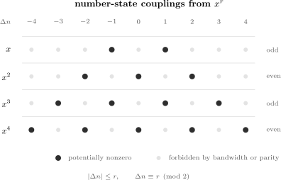
Potentially nonzero matrix elements of $x^r$ in the number basis. Polynomial degree fixes the matrix bandwidth, while parity fixes whether $\Delta n$ is even or odd.

The selection rule should be applied before expanding operator products. It predicts which energy corrections vanish, which intermediate states can appear, and how wide a numerical Hamiltonian matrix will be.

Normal-Ordering Shortcuts

Because $a$ and $a^\dagger$ do not commute, an ordinary binomial expansion of $(a+a^\dagger)^r$ is invalid. Normal ordering collects the commutator corrections. With colons denoting normal order,

$$q^2=:q^2:+1,$$ $$q^3=:q^3:+3q,$$

and

$$q^4=:q^4:+6:q^2:+3.$$

For a diagonal number-state matrix element, only terms with equal numbers of $a$ and $a^\dagger$ survive. For example,

$$\begin{aligned} \langle n\vert q^4\vert n\rangle ={}& 6n(n-1)+12n+3 \\ ={}& 6n^2+6n+3. \end{aligned}$$

These identities are the one-mode precursor of the normal-ordering and contraction bookkeeping used in many-body theory and quantum field theory.

Four Perturbations at a Glance

Use $\lambda$ only as an order-counting parameter and write

$$H(\lambda)=H_0+\lambda V.$$

$V$	First energy shift	First nonzero energy order	Exact or large-order lesson
$Fx$	zero	second	energy series terminates; exact displacement
$\kappa x^2$	nonzero	first	exact frequency change; finite Taylor radius
$\gamma x^3$	zero	second	real pure cubic is unbounded below
$g x^4$, $g\gt0$	nonzero	first	stable model; perturbative series is asymptotic

The same unperturbed basis therefore supports four distinct lessons. A zero first-order diagonal element can mean exact cancellation, delayed response, or an ill-posed global model; the order label alone does not decide which.

Linear Perturbation: Displacement

Let

$$V=Fx,$$

where $F$ has units of force. Parity immediately gives

$$E_n^{(1)} = F\langle n\vert x\vert n\rangle =0.$$

The first-order state correction has only neighboring levels:

$$\begin{aligned} \lvert n^{(1)}\rangle = \frac{F x_{\mathrm{zpf}}}{\hbar\omega} \Bigl[ &\sqrt n\,\lvert n-1\rangle \\ &- \sqrt{n+1}\,\lvert n+1\rangle \Bigr]. \end{aligned}$$

At second order,

$$\begin{aligned} E_n^{(2)} ={}& F^2x_{\mathrm{zpf}}^2 \left[ \frac{n}{\hbar\omega} - \frac{n+1}{\hbar\omega} \right] \\ ={}& -\frac{F^2}{2m\omega^2}. \end{aligned}$$

The cancellation of $n$ is a strong check. Every level receives the same shift, so the spacing remains $\hbar\omega$.

Completing the square gives the exact answer:

$$\begin{aligned} H(\lambda) ={}& \frac{p^2}{2m} + \frac{1}{2}m\omega^2 \left( x+\frac{\lambda F}{m\omega^2} \right)^2 \\ &- \frac{\lambda^2F^2}{2m\omega^2}. \end{aligned}$$

Hence

$$E_n(\lambda) = \hbar\omega \left(n+\frac{1}{2}\right) - \frac{\lambda^2F^2}{2m\omega^2}.$$

The energy expansion terminates at second order, even though the translated eigenstate contains all orders when expanded in the original number basis. Displaced Oscillator owns the exact coordinate, translation-operator, and coherent-state descriptions. First-Order State Corrections owns the detailed perturbative mixing analysis.

Quadratic Perturbation: Frequency Renormalization

Now take

$$V=\kappa x^2.$$

Applying $x^2=x_{\mathrm{zpf}}^2q^2$ to a number state gives

$$\begin{aligned} x^2\lvert n\rangle ={}& x_{\mathrm{zpf}}^2 \Bigl[ \\[-0.25em] &\sqrt{n(n-1)}\,\lvert n-2\rangle \\ &+ (2n+1)\lvert n\rangle \\ &+ \sqrt{(n+1)(n+2)}\,\lvert n+2\rangle \Bigr]. \end{aligned}$$

Therefore

$$\begin{aligned} E_n^{(1)} &= \kappa x_{\mathrm{zpf}}^2(2n+1) \\ &= \frac{\kappa\hbar}{m\omega} \left(n+\frac{1}{2}\right). \end{aligned}$$

The first-order state correction is

$$\begin{aligned} \lvert n^{(1)}\rangle ={}& \frac{\kappa x_{\mathrm{zpf}}^2} {2\hbar\omega} \Bigl[ \\[-0.25em] &\sqrt{n(n-1)}\,\lvert n-2\rangle \\ &- \sqrt{(n+1)(n+2)}\,\lvert n+2\rangle \Bigr]. \end{aligned}$$

Only the off-diagonal terms enter the second-order energy:

$$\begin{aligned} E_n^{(2)} ={}& \frac{\kappa^2x_{\mathrm{zpf}}^4} {2\hbar\omega} \Bigl[ n(n-1) \\ &\qquad{} - (n+1)(n+2) \Bigr] \\ ={}& -\frac{\kappa^2\hbar} {2m^2\omega^3} \left(n+\frac{1}{2}\right). \end{aligned}$$

This perturbation is exactly another harmonic oscillator:

$$\Omega(\lambda)^2 = \omega^2+\frac{2\lambda\kappa}{m}.$$

Thus

$$E_n(\lambda) = \hbar\Omega(\lambda) \left(n+\frac{1}{2}\right).$$

Expanding

$$\Omega(\lambda) = \omega \sqrt{ 1+\frac{2\lambda\kappa}{m\omega^2} }$$

reproduces $E_n^{(1)}$ and $E_n^{(2)}$. The exact state has a changed width and is a squeezed number state relative to the original oscillator basis. Squeezed States: First Encounter supplies the state-space language.

Stability requires

$$\omega^2+\frac{2\lambda\kappa}{m}\gt0.$$

The Taylor series about $\lambda=0$ has a branch point where the effective frequency vanishes. For the binomial expansion, the nearest such point sets the radius

$$\left| \frac{2\lambda\kappa}{m\omega^2} \right| \lt1.$$

The exact oscillator can remain stable at some parameter values outside that Taylor disk; exact solvability and convergence of one chosen expansion are different questions.

Cubic Perturbation: Symmetry and Stability

Let

$$V=\gamma x^3.$$

Because $x^3$ is odd,

$$E_n^{(1)} = \gamma\langle n\vert x^3\vert n\rangle =0.$$

The action of $q^3$ is

$$\begin{gathered} q^3\lvert n\rangle = \\[-0.25em] \begin{aligned} & \sqrt{n(n-1)(n-2)} \lvert n-3\rangle \\ &+ 3n\sqrt n\,\lvert n-1\rangle \\ &+ 3(n+1)\sqrt{n+1}\, \lvert n+1\rangle \\ &+ \sqrt{(n+1)(n+2)(n+3)} \lvert n+3\rangle. \end{aligned} \end{gathered}$$

The four allowed channels give the formal second-order coefficient

$$\begin{aligned} E_n^{(2)} = -\frac{ \gamma^2x_{\mathrm{zpf}}^6 }{ \hbar\omega } \bigl( 30n^2+30n+11 \bigr). \end{aligned}$$

For the ground state,

$$E_0^{(2)} = -\frac{ 11\gamma^2x_{\mathrm{zpf}}^6 }{ \hbar\omega }.$$

The vanishing first-order shift therefore does not mean that the cubic term has no spectral effect.

There is, however, a global caveat. The real potential

$$\frac{1}{2}m\omega^2x^2+\lambda\gamma x^3$$

is unbounded below on one side for every nonzero real $\lambda\gamma$. It does not define a stable bound-state oscillator on the full line. The coefficients above are formal local perturbative data and can be connected to resonance problems under additional analytic prescriptions; they should not be advertised as convergent corrections to a stable bound spectrum.

A physically stable asymmetric well needs stabilizing higher powers, a restricted effective domain, or a more complete potential. This is a case where symmetry algebra can be correct while the global Hamiltonian model is incomplete.

Quartic Perturbation: Stable Anharmonicity

Take

$$V=gx^4, \qquad g\gt0.$$

Normal ordering gives

$$\langle n\vert x^4\vert n\rangle = x_{\mathrm{zpf}}^4 \bigl( 6n^2+6n+3 \bigr).$$

Hence

$$\begin{aligned} E_n^{(1)} ={}& 3g x_{\mathrm{zpf}}^4 \bigl( 2n^2+2n+1 \bigr) \\ ={}& \frac{3g\hbar^2} {4m^2\omega^2} \bigl( 2n^2+2n+1 \bigr). \end{aligned}$$

For the ground state, the first two coefficients are

$$\begin{aligned} E_0(\lambda) ={}& \frac{\hbar\omega}{2} + 3\lambda g x_{\mathrm{zpf}}^4 \\ &- \frac{ 42\lambda^2g^2x_{\mathrm{zpf}}^8 }{ \hbar\omega } + O(\lambda^3). \end{aligned}$$

The number $42$ comes from the two off-diagonal channels $\lvert2\rangle$ and $\lvert4\rangle$. The complete derivation belongs to Anharmonic Oscillator by Perturbation Theory.

Unlike the pure real cubic model, the potential is bounded below for $g\gt0$. Yet stability does not imply a convergent Rayleigh–Schrödinger series. The quartic-oscillator coefficients grow factorially at high order; low orders are useful for weak coupling, while the full series requires asymptotic and resummation ideas.

Anharmonic Oscillator is the canonical multi-method comparison among perturbative, variational, semiclassical, and numerical descriptions.

Dimensionless Control Parameters

For a monomial

$$V_r=c_r x^r,$$

define the low-state dimensionless coupling

$$g_r \equiv \frac{ c_r x_{\mathrm{zpf}}^r }{ \hbar\omega }.$$

At number $n$, matrix elements of $q^r$ grow parametrically as $n^{r/2}$ along allowed channels. A conservative mixing estimate is therefore

$$\lvert\lambda g_r\rvert n^{r/2} \ll1,$$

up to order-one coefficients and the allowed value of $\Delta n$. This estimate is not a universal error bound, but it makes one failure mode visible: a coupling that is perturbative for the ground state may not be perturbative high in the spectrum.

Different observables can have different effective criteria:

• eigenvector mixing compares off-diagonal matrix elements with level gaps;
• energy accuracy compares omitted corrections with the requested energy scale;
• transition amplitudes can be sensitive to small state admixtures;
• a near cancellation can make relative error misleading even when absolute error is small.

The exactly solvable linear and quadratic cases should be used to calibrate any proposed error diagnostic.

Matrix Structure and Numerical Checks

In the number basis, a polynomial of degree $r$ produces a banded matrix:

$$\langle m\vert x^r\vert n\rangle=0 \qquad \text{if } \lvert m-n\rvert\gt r.$$

Parity sharpens the structure:

• even potentials preserve even and odd sectors separately;
• odd potentials couple the two parity sectors;
• $x^4$ requires only the five bands $\Delta n=0,\pm2,\pm4$;
• a sum of monomials has the union of their allowed bands.

For a basis truncated at $n\le N_{\max}$, test:

1. convergence of target eigenvalues as $N_{\max}$ increases;
2. residual norms of the computed eigenpairs;
3. stability of perturbative coefficients fitted at small $\lambda$;
4. parity-block consistency when the Hamiltonian is even;
5. sensitivity to the reference frequency used to define the basis.

A basis with an optimized reference frequency can converge much faster for a strongly broadened or narrowed state. That is a basis choice, not a change in the physical Hamiltonian.

Variational Comparison

The oscillator examples clarify what a Gaussian trial family can and cannot do.

• Linear force: a displaced Gaussian is the exact ground state.
• Quadratic change: a Gaussian with adjustable width is the exact ground state of the new frequency.
• Stable quartic term: an optimized Gaussian gives an upper bound but cannot reproduce the exact non-Gaussian tails.
• Pure real cubic term: no variational ground-state minimum exists because the potential is unbounded below.

For the quartic oscillator, a trial frequency $\Omega$ resums selected effects of $g$ into the reference state. Expanding the optimized result at weak coupling can reproduce low-order trends, while its finite-coupling behavior answers a different variational question. Variational Perturbation Theory promotes that frequency to an order-dependent reference scale and derives the formal δ re-expansion. Compare methods at equal physical parameters, not merely by the number of algebraic terms retained.

See Variational Principle for the bound and stationarity logic.

Bridge to Quantum Field Theory

Each free-field normal mode is a harmonic oscillator, and a field operator is a sum of mode coordinates proportional to $a_{\mathbf k}+a_{\mathbf k}^\dagger$. Polynomial field interactions therefore generate products of creation and annihilation operators much as $x^3$ and $x^4$ do here.

The analogy teaches several durable habits:

• normal order noncommuting products rather than using a classical binomial expansion;
• use selection rules before summing intermediate states;
• distinguish diagonal shifts from state-changing terms;
• expect disconnected and contraction terms at higher order;
• check whether the perturbative series is convergent or only asymptotic.

One oscillator does not contain spatial locality, momentum conservation among modes, ultraviolet divergences, renormalization, or infinitely many degrees of freedom. The bridge is structural, not an equivalence. Harmonic Oscillator to Quantum Fields and Normal Ordering continue the comparison.

Practical Workflow

1. Fix the oscillator-length convention. Write $x$ in terms of $a+a^\dagger$ before computing coefficients.
2. Classify parity and degree. List allowed $\Delta n$ values.
3. Identify the leading nonzero order. A vanishing diagonal term shifts attention to state response and second order.
4. Check global stability. A locally small perturbation can make the full potential unbounded.
5. Exploit exact reorganizations. Displace a linear term or redefine the frequency for a quadratic term.
6. Form a dimensionless coupling. Include the oscillator width and the state number.
7. Cross-check coefficients. Expand an exact result, use parity, or compare with numerical diagonalization.
8. State the series meaning. Distinguish terminating, convergent, formal, and asymptotic expansions.

Common Mistakes

• Using $x_{\mathrm{zpf}}=\sqrt{\hbar/(m\omega)}$ while also writing $x=x_{\mathrm{zpf}}(a+a^\dagger)$.
• Expanding $(a+a^\dagger)^r$ as though $a$ and $a^\dagger$ commute.
• Concluding that an odd perturbation has no effect because its first-order energy vanishes.
• Forgetting the lower-state terms with positive denominators in an excited-state second-order sum.
• Calling the pure real cubic oscillator a stable bound-state problem.
• Treating the exact quadratic frequency change as proof that every perturbation series converges.
• Assuming a weak coupling for $n=0$ remains weak at large $n$.
• Duplicating the quartic model calculation instead of linking its canonical worked and multi-method pages.
• Trusting a truncated oscillator basis without varying its cutoff or reference frequency.

Exercises

1. Prove the polynomial selection rule

Show that $\langle m\vert x^r\vert n\rangle$ can be nonzero only when $\lvert m-n\rvert\le r$ and $m-n$ has the same parity as $r$.

Solution

Since

$$x^r = x_{\mathrm{zpf}}^r (a+a^\dagger)^r,$$

every ordered term contains $r$ ladder operations. If a term contains $u$ creation operators and $r-u$ annihilation operators, its net number change is

$$\Delta n = u-(r-u) = 2u-r.$$

Therefore

$$\lvert\Delta n\rvert\le r$$

and

$$\Delta n\equiv r\pmod2.$$

Commuting operators into normal order removes pairs through $[a,a^\dagger]=1$, changing the degree by two and preserving the same parity condition.

2. Verify the linear exact check

Starting from the sum-over-states formula, compute the second-order energy for $V=Fx$ and show that it equals the exact displaced-oscillator shift.

Solution

Only $m=n\pm1$ contribute:

$$\begin{aligned} E_n^{(2)} ={}& \frac{ F^2x_{\mathrm{zpf}}^2 n }{ \hbar\omega } \\ &- \frac{ F^2x_{\mathrm{zpf}}^2(n+1) }{ \hbar\omega }. \end{aligned}$$

Thus

$$E_n^{(2)} = -\frac{ F^2x_{\mathrm{zpf}}^2 }{ \hbar\omega } = -\frac{F^2}{2m\omega^2}.$$

Completing the square gives an exact constant offset

$$-\frac{\lambda^2F^2}{2m\omega^2},$$

so the perturbative result is exact and independent of $n$.

3. Match the quadratic expansion

Expand the exact frequency

$$\Omega(\lambda) = \sqrt{ \omega^2+\frac{2\lambda\kappa}{m} }$$

through second order and recover $E_n^{(1)}$ and $E_n^{(2)}$.

Solution

Factor out $\omega$:

$$\Omega(\lambda) = \omega \sqrt{ 1+\frac{2\lambda\kappa}{m\omega^2} }.$$

Using $\sqrt{1+z}=1+z/2-z^2/8+O(z^3)$,

$$\begin{aligned} \Omega(\lambda) ={}& \omega + \lambda\frac{\kappa}{m\omega} \\ &- \lambda^2 \frac{\kappa^2}{2m^2\omega^3} + O(\lambda^3). \end{aligned}$$

Multiplication by $\hbar(n+1/2)$ gives

$$E_n^{(1)} = \frac{\kappa\hbar}{m\omega} \left(n+\frac{1}{2}\right)$$

and

$$E_n^{(2)} = -\frac{\kappa^2\hbar}{2m^2\omega^3} \left(n+\frac{1}{2}\right).$$

4. Compute the cubic ground-state coefficient

For $V=\gamma x^3$, use $q^3\lvert0\rangle$ to compute $E_0^{(2)}$. Then state why the result requires a stability caveat.

Solution

The cubic action on the ground state is

$$q^3\lvert0\rangle = 3\lvert1\rangle + \sqrt6\,\lvert3\rangle.$$

Therefore

$$\begin{aligned} E_0^{(2)} ={}& \gamma^2x_{\mathrm{zpf}}^6 \left[ \frac{9}{-\hbar\omega} + \frac{6}{-3\hbar\omega} \right] \\ ={}& -\frac{ 11\gamma^2x_{\mathrm{zpf}}^6 }{ \hbar\omega }. \end{aligned}$$

The algebra is correct as a formal local coefficient, but a real $x^3$ term makes the potential unbounded below on one side. A stable global model needs additional stabilizing structure.

5. Derive the quartic diagonal element

Use

$$q^4=:q^4:+6:q^2:+3$$

to derive $\langle n\vert q^4\vert n\rangle$.

Solution

In $:q^4:$, only the term with two creation and two annihilation operators is diagonal:

$$\begin{aligned} \langle n\vert:q^4:\vert n\rangle &= 6 \langle n\vert (a^\dagger)^2a^2 \vert n\rangle \\ &= 6n(n-1). \end{aligned}$$

In $:q^2:$, the only diagonal term is $2a^\dagger a$, so

$$6\langle n\vert:q^2:\vert n\rangle = 12n.$$

Adding the contraction constant gives

$$\begin{aligned} \langle n\vert q^4\vert n\rangle &= 6n(n-1)+12n+3 \\ &= 6n^2+6n+3. \end{aligned}$$

6. Design a parity-resolved numerical matrix

For $H=H_0+gx^4$, explain how parity and bandwidth reduce a matrix calculation in the number basis. What convergence checks remain necessary?

Solution

$x^4$ connects only

$$\Delta n=0,\pm2,\pm4.$$

The Hamiltonian therefore separates into an even block built from

$$\lvert0\rangle,\lvert2\rangle,\lvert4\rangle,\ldots$$

and an odd block built from

$$\lvert1\rangle,\lvert3\rangle,\lvert5\rangle,\ldots.$$

Within either block the matrix is banded, so forbidden entries need not be stored or computed. One must still increase the maximum number state, monitor eigenpair residuals, check target eigenvalue stability, and test whether a different reference frequency improves convergence. Parity reduces cost but does not control truncation error by itself.

Cross-Links

• Quantum Harmonic Oscillator for the exact reference model.
• Ladder-Operator Solution for the spectrum and ladder algebra.
• First-Order Energy Corrections for diagonal response and symmetry.
• First-Order State Corrections for induced mixing and the linear-force example.
• Second-Order Energy Corrections for denominator signs and virtual transitions.
• Sum Rules and Completeness Tricks for oscillator sum checks.
• Displaced Oscillator for the exact linear perturbation.
• Anharmonic Oscillator for the durable multi-method quartic model.
• Anharmonic Oscillator by Perturbation Theory for the detailed quartic calculation.
• Matrix Diagonalization for numerical eigenpair and residual checks.

References

• J. J. Sakurai and J. Napolitano, Modern Quantum Mechanics, 3rd ed., Cambridge University Press, 2021, Chapter 5.
• C. Cohen-Tannoudji, B. Diu, and F. Laloë, Quantum Mechanics, Vol. I, Wiley, 1977, oscillator complements; Vol. II, perturbation theory.
• R. Shankar, Principles of Quantum Mechanics, 2nd ed., Springer, 1994, Chapters 7 and 17.
• A. Messiah, Quantum Mechanics, Vol. II, North-Holland, 1962, Chapter XVII.
• C. M. Bender and T. T. Wu, “Anharmonic Oscillator,” Physical Review 184, 1231–1260 (1969), doi:10.1103/PhysRev.184.1231.
• C. M. Bender and T. T. Wu, “Anharmonic Oscillator. II. A Study of Perturbation Theory in Large Order,” Physical Review D 7, 1620–1636 (1973), doi:10.1103/PhysRevD.7.1620.
• B. Simon, “Coupling Constant Analyticity for the Anharmonic Oscillator,” Annals of Physics 58, 76–136 (1970), doi:10.1016/0003-4916(70)90240-X.
• J. Zinn-Justin, Quantum Field Theory and Critical Phenomena, 4th ed., Oxford University Press, 2002.