Second-Order Energy Corrections

The second-order energy correction is the leading energy effect of off-diagonal mixing. For an isolated nondegenerate eigenvalue of

$$H(\lambda)=H_0+\lambda V,$$

Rayleigh–Schrödinger perturbation theory gives

$$E_n^{(2)} = \sum_{m\ne n} \frac{ \left| \langle m^{(0)}\rvert V \lvert n^{(0)}\rangle \right|^2 }{ E_n^{(0)}-E_m^{(0)} }.$$

The actual quadratic contribution to the energy is $\lambda^2E_n^{(2)}$. Each term combines a transition strength with a signed inverse energy gap. Coupling to a higher level pushes the target level down; coupling to a lower level pushes it up. This is the perturbative form of level repulsion.

This page owns the detailed interpretation, sign analysis, ground-state result, static-polarizability connection, and convergence diagnostics for the formula. The order-by-order framework is introduced on Nondegenerate Perturbation Theory, while extended model calculations keep their own canonical homes.

Result at a Glance

Assume

$$\begin{aligned} H_0\lvert n^{(0)}\rangle &= E_n^{(0)}\lvert n^{(0)}\rangle, \\ \langle n^{(0)}\vert n^{(0)}\rangle &=1, \end{aligned}$$

where $E_n^{(0)}$ is a simple isolated eigenvalue. Expand the corresponding eigenvalue branch as

$$E_n(\lambda) = E_n^{(0)} +\lambda E_n^{(1)} +\lambda^2E_n^{(2)} +O(\lambda^3).$$

For a Hamiltonian linear in $\lambda$,

$$\begin{aligned} E_n^{(1)} &= \langle n^{(0)}\rvert V \lvert n^{(0)}\rangle, \\ E_n^{(2)} &= \sum_{m\ne n} \frac{ \left|V_{mn}\right|^2 }{ E_n^{(0)}-E_m^{(0)} }, \end{aligned}$$

with

$$V_{mn} \equiv \langle m^{(0)}\rvert V \lvert n^{(0)}\rangle.$$

The formula requires more than a formally small $\lambda$:

• the target eigenvalue must be isolated from levels that are being treated one at a time;
• the ratios $\lvert\lambda V_{mn}\rvert/\lvert E_n^{(0)}-E_m^{(0)}\rvert$ must be small for materially coupled states;
• the sum, including any continuum contribution, must exist in the intended operator or quadratic-form setting;
• the basis in the sum must be complete in the relevant symmetry sector.

If the Hamiltonian itself contains a quadratic term,

$$H(\lambda) = H_0+\lambda V+\lambda^2W+O(\lambda^3),$$

then the result becomes

$$E_n^{(2)} = \langle n^{(0)}\rvert W \lvert n^{(0)}\rangle + \sum_{m\ne n} \frac{ \left|V_{mn}\right|^2 }{ E_n^{(0)}-E_m^{(0)} }.$$

The expectation of $W$ is an explicit second-order contribution. It is conceptually distinct from the mixing term generated by applying $V$ twice.

Derivation from the Eigenvalue Equation

Use intermediate normalization,

$$\langle n^{(0)}\vert n(\lambda)\rangle=1,$$

and write

$$\begin{aligned} \lvert n(\lambda)\rangle ={}& \lvert n^{(0)}\rangle +\lambda\lvert n^{(1)}\rangle \\ &+ \lambda^2\lvert n^{(2)}\rangle +O(\lambda^3), \\ E_n(\lambda) ={}& E_n^{(0)} +\lambda E_n^{(1)} \\ &+ \lambda^2E_n^{(2)} +O(\lambda^3). \end{aligned}$$

The first-order equation is

$$\bigl(H_0-E_n^{(0)}\bigr) \lvert n^{(1)}\rangle = - \bigl(V-E_n^{(1)}\bigr) \lvert n^{(0)}\rangle.$$

Projecting onto $\langle m^{(0)}\rvert$ for $m\ne n$ gives

$$\langle m^{(0)}\vert n^{(1)}\rangle = \frac{V_{mn}} {E_n^{(0)}-E_m^{(0)}}.$$

The coefficient of $\lambda^2$ in the eigenvalue equation is

$$\begin{aligned} \bigl(H_0-E_n^{(0)}\bigr) \lvert n^{(2)}\rangle ={}& - \bigl(V-E_n^{(1)}\bigr) \lvert n^{(1)}\rangle \\ &+ E_n^{(2)} \lvert n^{(0)}\rangle. \end{aligned}$$

Left-multiplying by $\langle n^{(0)}\rvert$ removes the $H_0-E_n^{(0)}$ term. Intermediate normalization also gives

$$\langle n^{(0)}\vert n^{(1)}\rangle=0,$$

so

$$E_n^{(2)} = \langle n^{(0)}\rvert V \lvert n^{(1)}\rangle.$$

Inserting the spectral expansion of $\lvert n^{(1)}\rangle$ yields the sum-over-states formula. The diagonal matrix element $V_{nn}$ does not appear in that sum because it generated $E_n^{(1)}$ and was removed by the orthogonal projection.

This derivation also explains why phase and normalization choices do not alter $E_n^{(2)}$. They change the component of $\lvert n^{(1)}\rangle$ parallel to $\lvert n^{(0)}\rangle$, but the consistently normalized eigenvalue coefficient is invariant.

Projector and Resolvent Form

Define the spectral projectors

$$\begin{aligned} P_n &= \lvert n^{(0)}\rangle \langle n^{(0)}\rvert, \\ Q_n &=I-P_n. \end{aligned}$$

On the orthogonal complement of the target state, define the reduced resolvent

$$R_n' \equiv Q_n \frac{1}{E_n^{(0)}-H_0} Q_n.$$

Its spectral representation is

$$R_n' = \sum_{m\ne n} \frac{ \lvert m^{(0)}\rangle \langle m^{(0)}\rvert }{ E_n^{(0)}-E_m^{(0)} },$$

with continuum integrals added where required. Then

$$\begin{aligned} \lvert n^{(1)}\rangle &= R_n'V\lvert n^{(0)}\rangle, \\ E_n^{(2)} &= \langle n^{(0)}\rvert V R_n' V \lvert n^{(0)}\rangle. \end{aligned}$$

This form separates three ingredients:

1. $V\lvert n^{(0)}\rangle$ creates amplitudes outside the reference state.
2. $R_n'$ weights those amplitudes by signed inverse energy gaps.
3. The second $V$ returns them to the reference sector.

The resolvent notation becomes especially useful in effective-Hamiltonian methods, response theory, and calculations that avoid an explicit spectral sum. The canonical operator treatment is Resolvent Operator.

Virtual Mixing and Level Repulsion

The phrase virtual mixing describes the intermediate-state structure of the calculation. The target state acquires an amplitude proportional to $V_{mn}/(E_n^{(0)}-E_m^{(0)})$, and acting with $V$ again converts that amplitude into an energy correction.

Nothing in this stationary derivation describes a particle literally occupying $\lvert m^{(0)}\rangle$ for a measurable interval. The intermediate states are components of the perturbed eigenvector, or equivalently terms in a resolvent expansion. Calling them virtual is useful bookkeeping language, not a claim about a hidden time-resolved trajectory.

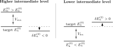
Coupling to a higher unperturbed level gives a negative contribution to the target energy, while coupling to a lower level gives a positive contribution. A ground state has no lower levels, so its mixing correction cannot be positive.

For a two-level Hamiltonian

$$\begin{aligned} H(\lambda) &= \begin{pmatrix} E_a & \lambda v \\ \lambda v^* & E_b \end{pmatrix}, \\ \Delta &\equiv E_b-E_a\gt0. \end{aligned}$$

the exact eigenvalues are

$$E_\pm = \frac{E_a+E_b}{2} \pm \frac12 \sqrt{\Delta^2+4\lambda^2\lvert v\rvert^2}.$$

Expanding at small $\lambda$ gives

$$\begin{aligned} E_-(\lambda) &= E_a -\lambda^2 \frac{\lvert v\rvert^2}{\Delta} +O(\lambda^4), \\ E_+(\lambda) &= E_b +\lambda^2 \frac{\lvert v\rvert^2}{\Delta} +O(\lambda^4). \end{aligned}$$

The lower level moves down and the upper level moves up. The same exact expression also exposes the control condition $\lvert\lambda v\rvert/\Delta\ll1$. When the gap is comparable to the coupling, expanding the square root is no longer justified.

Sign Structure

Partition the intermediate spectrum into states below and above the target energy:

$$\begin{aligned} \mathcal L_n &= \{m:E_m^{(0)}\lt E_n^{(0)}\}, \\ \mathcal U_n &= \{m:E_m^{(0)}\gt E_n^{(0)}\}. \end{aligned}$$

For an isolated nondegenerate target,

$$\begin{aligned} E_n^{(2)} ={}& \sum_{m\in\mathcal L_n} \frac{ \lvert V_{mn}\rvert^2 }{ E_n^{(0)}-E_m^{(0)} } \\ &- \sum_{m\in\mathcal U_n} \frac{ \lvert V_{mn}\rvert^2 }{ E_m^{(0)}-E_n^{(0)} }. \end{aligned}$$

The consequences are immediate.

Target level	Sign information
Nondegenerate ground state	$E_0^{(2)}\le0$
Highest level of a finite-dimensional system	$E_{\max}^{(2)}\ge0$
Generic excited state	No fixed sign; lower and upper states compete
State uncoupled off-diagonally by $V$	Mixing contribution vanishes
Nearly degenerate state	Sign may be apparent, but the nondegenerate expansion is not controlled

For the ground state,

$$E_0^{(2)} = - \sum_{m\ne0} \frac{ \lvert V_{m0}\rvert^2 }{ E_m^{(0)}-E_0^{(0)} } \le0.$$

Equality holds precisely when the perturbation has no component that connects the ground state to its orthogonal complement:

$$Q_0V\lvert0^{(0)}\rangle=0.$$

This includes, but is not limited to, the case where $\lvert0^{(0)}\rangle$ is an eigenstate of $V$. A zero second-order mixing correction does not imply that the first-order shift vanishes.

Why the Ground State Moves Down

The sign theorem has a variational interpretation. The exact ground-state energy is

$$E_0(\lambda) = \inf_{\langle\psi\vert\psi\rangle=1} \langle\psi\rvert H_0+\lambda V \lvert\psi\rangle.$$

For each fixed normalized trial state, the expectation value is affine in $\lambda$. The infimum of affine functions is concave. Therefore, wherever the isolated ground-state branch is twice differentiable,

$$\frac{d^2E_0}{d\lambda^2}\le0.$$

Because

$$\left. \frac{d^2E_0}{d\lambda^2} \right|_{\lambda=0} = 2E_0^{(2)},$$

the perturbative sign follows. Equivalently, using the unperturbed ground state as a trial state gives the tangent-line bound

$$E_0(\lambda) \le E_0^{(0)} +\lambda \langle0^{(0)}\rvert V \lvert0^{(0)}\rangle.$$

The true ground state can lower its energy by adjusting its wavefunction, and the first gain from that adjustment is the nonpositive mixing correction. This argument concerns the lowest eigenvalue. It does not impose concavity on each excited-state branch. See Variational Principle for the canonical bound-based method.

Static Polarizability

Let a static electric field $\boldsymbol{\mathcal E}$ couple to a dipole operator $\mathbf D$ through

$$H(\boldsymbol{\mathcal E}) = H_0 - \boldsymbol{\mathcal E}\mathbin{\cdot}\mathbf D.$$

For a nondegenerate state with no permanent dipole in the chosen direction, the energy expansion begins as

$$E_n(\boldsymbol{\mathcal E}) = E_n(0) - \frac12 \alpha_{ij}^{(n)} \mathcal E_i\mathcal E_j +O(\mathcal E^3).$$

Comparing with the second-order perturbative sum gives the symmetric static-polarizability tensor

$$\begin{aligned} \alpha_{ij}^{(n)} ={}& 2\operatorname{Re} \sum_{m\ne n} \frac{ \langle n\rvert D_i\lvert m\rangle \langle m\rvert D_j\lvert n\rangle }{ E_m-E_n }. \end{aligned}$$

Along a unit vector $\mathbf e$,

$$\alpha_{\mathbf e}^{(n)} = 2 \sum_{m\ne n} \frac{ \left| \langle m\rvert \mathbf e\mathbin{\cdot}\mathbf D \lvert n\rangle \right|^2 }{ E_m-E_n }.$$

For a nondegenerate ground state, every denominator is positive, so $\alpha_{\mathbf e}^{(0)}\ge0$. The corresponding energy shift is nonpositive:

$$\Delta E_0 = -\frac12 \alpha_{\mathbf e}^{(0)} \mathcal E^2 +O(\mathcal E^3).$$

For an excited state, lower levels contribute with the opposite sign and the static coefficient need not be positive. Degeneracies require diagonalizing the dipole interaction in the degenerate subspace, and a frequency-dependent field requires dynamical response rather than the static formula. Parity often removes the permanent dipole and restricts the sum to opposite-parity states. See Stark Effect as a Perturbation Example for the method decision and Selection Rules for the symmetry logic.

Sum-over-States Forms

When $H_0$ has both discrete and continuum spectrum, a schematic spectral resolution gives

$$\begin{aligned} E_n^{(2)} ={}& \sum_{m\in\mathrm{disc}\atop m\ne n} \frac{ \lvert V_{mn}\rvert^2 }{ E_n^{(0)}-E_m^{(0)} } \\ &+ \sum_c \int_{E_{c,\mathrm{th}}}^{\infty} dE\, \frac{ \left| \langle E,c\rvert V \lvert n^{(0)}\rangle \right|^2 }{ E_n^{(0)}-E }. \end{aligned}$$

Here $c$ labels continuum channels, and the normalization convention for $\lvert E,c\rangle$ determines the measure. For a bound target below all included thresholds, the continuum denominator never vanishes. For an embedded state or a target above an open threshold, poles and decay channels signal that ordinary bound-state perturbation theory is not the complete framework. Principal values, outgoing boundary conditions, self-energies, or resonance theory may be required.

Completeness by itself removes an unweighted sum such as

$$\sum_m \lvert V_{mn}\rvert^2,$$

but it does not remove the energy denominator. Exact commutator identities, controlled closure approximations, or an inhomogeneous equation can sometimes replace the explicit sum. Those methods belong on Sum Rules and Completeness Tricks.

Computing Without Listing Every State

Define $\lvert\chi_n\rangle$ by the projected equation

$$\begin{aligned} \bigl(H_0-E_n^{(0)}\bigr) \lvert\chi_n\rangle &= -Q_nV\lvert n^{(0)}\rangle, \\ \langle n^{(0)}\vert\chi_n\rangle &=0. \end{aligned}$$

Then

$$\lvert\chi_n\rangle = R_n'V\lvert n^{(0)}\rangle = \lvert n^{(1)}\rangle,$$

and

$$E_n^{(2)} = \langle n^{(0)}\rvert V \lvert\chi_n\rangle.$$

This Dalgarno–Lewis strategy can be preferable when the intermediate spectrum is infinite, includes continuum states, or is inconvenient to construct explicitly. In a numerical basis, the linear system must be solved only on the $Q_n$ subspace; otherwise the singular null direction along $\lvert n^{(0)}\rangle$ makes the equation nonunique.

Completeness and Convergence

A formally correct summand does not guarantee a meaningful sum. Several distinct questions must be checked.

Spectral completeness

The inserted identity must include every discrete state, continuum channel, internal degree of freedom, and symmetry sector reached by $V$. Selection rules may remove sectors exactly, but omission by convenience is not a selection rule.

High-energy convergence

At large intermediate energy, the decay of matrix elements must overcome the density of states and the inverse-gap factor. For unbounded perturbations, convergence may depend on operator domains or quadratic-form bounds. A divergent expression is not repaired by merely calling $\lambda$ small.

Near-degenerate denominators

A single small denominator can dominate the sum and simultaneously invalidate it. If

$$\frac{ \lvert\lambda V_{mn}\rvert }{ \lvert E_n^{(0)}-E_m^{(0)}\rvert } \not\ll1,$$

the corresponding states should usually be treated as a joint model space. Use Degenerate Perturbation Theory even when the levels are only nearly degenerate.

Numerical truncation

For a truncated sum, report how the estimate changes as the energy cutoff or basis size increases. Useful diagnostics include:

• checking exact selection rules before summing;
• tracking contributions by energy window rather than only the final total;
• comparing the direct sum with the projected linear solve;
• testing unweighted and energy-weighted sum rules;
• verifying dimensions and the expected sign when a sign theorem applies;
• comparing with direct diagonalization at several small values of $\lambda$.

For a ground state, every exact intermediate-state contribution is nonpositive. In a literal partial spectral sum, adding more exact states can only make $E_0^{(2)}$ more negative. This monotonicity need not survive arbitrary basis approximations in which both energies and matrix elements change as the basis is enlarged.

Worked Example: A Quadratic Oscillator Perturbation

Consider

$$H(\lambda) = \frac{P^2}{2m} +\frac12m\omega^2X^2 +\lambda\frac12m\Omega^2X^2,$$

where $\Omega^2$ sets the curvature added per unit $\lambda$. The exact Hamiltonian is another harmonic oscillator with frequency

$$\omega_\lambda = \sqrt{\omega^2+\lambda\Omega^2}.$$

We can therefore test perturbation theory against an exact answer.

Let

$$X = \sqrt{\frac{\hbar}{2m\omega}} \left(a+a^\dagger\right).$$

The perturbing operator is

$$\begin{aligned} V &= \frac12m\Omega^2X^2 \\ &= c \left( a^2+a^{\dagger2}+2a^\dagger a+1 \right), \end{aligned}$$

with

$$c \equiv \frac{\hbar\Omega^2}{4\omega}.$$

The diagonal element gives

$$E_n^{(1)} = c(2n+1) = \frac{\hbar\Omega^2}{2\omega} \left(n+\frac12\right).$$

Only the states $\lvert n-2\rangle$ and $\lvert n+2\rangle$ enter the second-order sum. Their matrix elements are

$$\begin{aligned} V_{n-2,n} &= c\sqrt{n(n-1)}, \\ V_{n+2,n} &= c\sqrt{(n+1)(n+2)}. \end{aligned}$$

Using the oscillator gaps gives

$$\begin{aligned} E_n^{(2)} ={}& c^2 \left[ \frac{n(n-1)}{2\hbar\omega} - \frac{(n+1)(n+2)}{2\hbar\omega} \right] \\ ={}& - \frac{\hbar\Omega^4}{8\omega^3} \left(n+\frac12\right). \end{aligned}$$

The lower intermediate state contributes positively and the upper one negatively. The upper-state matrix element is larger, so the net correction is negative for every $n$.

Now expand the exact frequency:

$$\omega_\lambda = \omega +\lambda\frac{\Omega^2}{2\omega} -\lambda^2\frac{\Omega^4}{8\omega^3} +O(\lambda^3).$$

The exact spectrum

$$E_n(\lambda) = \hbar\omega_\lambda \left(n+\frac12\right)$$

reproduces both perturbative coefficients. This example checks the denominators, ladder-operator factors, and sign competition without relying on perturbation theory for the final answer.

For the standard quartic oscillator, the complete first- and second-order ground-state calculation is kept on Anharmonic Oscillator by Perturbation Theory. Its result is a useful test of the same formula, but duplicating that derivation here would obscure its canonical home.

Boundaries of the Formula

The textbook expression should not be used unchanged in the following situations.

Situation	What changes
Exact degeneracy	Diagonalize $PVP$ within the degenerate subspace first.
Near degeneracy	Use a multi-state effective Hamiltonian or exact subspace diagonalization.
Embedded level or open decay channel	Bound-state eigenvalue perturbation may become resonance or self-energy theory.
Explicit $\lambda^2W$ in the Hamiltonian	Add $\langle W\rangle_n$ to the mixing contribution.
Unbounded or singular $V$	Establish a common operator domain or controlled quadratic-form setting.
Large order in an asymptotic series	Truncation error is not inferred from the next formal power alone.
Parameter-dependent basis	Include derivative or basis-change terms consistently rather than inserting the fixed-basis formula blindly.

When $[H_0,V]=0$ and the target is a nondegenerate common eigenstate, every off-diagonal $V_{mn}$ vanishes. The spectrum may shift linearly, but the second-order mixing term is zero. This is a useful check, not a failure of perturbation theory.

Practical Workflow

1. Write the Hamiltonian as a power series and identify whether an explicit $W$ term exists.
2. Specify the isolated unperturbed eigenvalue and its symmetry quantum numbers.
3. Compute or constrain $V_{mn}$ using Hermiticity and selection rules.
4. Inspect coupling-to-gap ratios before trusting any denominator.
5. Separate contributions from lower levels, upper levels, and continuum channels.
6. Evaluate the spectral sum or solve the projected inhomogeneous equation.
7. Check units, Hermitian conjugation, sign theorems, and convergence under cutoff enlargement.
8. Compare with exact diagonalization or a known limiting case whenever possible.

The answer should be reported as

$$E_n(\lambda) = E_n^{(0)} +\lambda E_n^{(1)} +\lambda^2E_n^{(2)} +O(\lambda^3),$$

not as an isolated coefficient with the power of $\lambda$ left ambiguous.

Common Mistakes

• Including $m=n$ in the spectral sum and creating a spurious zero denominator.
• Forgetting the square modulus when $V$ has complex matrix elements.
• Using perturbed energies in denominators while claiming a Rayleigh–Schrödinger result at fixed order.
• Calling the sign of an excited-state correction obvious without separating lower and upper intermediate states.
• Claiming that every second-order correction is negative; only the nondegenerate ground-state mixing term has that general sign.
• Omitting an explicit $\lambda^2W$ contribution from the Hamiltonian.
• Treating a tiny energy denominator as a large but valid correction rather than a warning that the expansion has failed.
• Summing only discrete states when continuum states are part of the completeness relation.
• Applying static polarizability formulas to resonant or time-dependent driving.
• Reporting a truncated numerical sum without a cutoff or basis-convergence test.
• Interpreting virtual intermediate states as hidden, directly occupied trajectories.

Exercises

1. Suppose $H(\lambda)=H_0+\lambda V+\lambda^2W$. Derive the second-order energy coefficient for an isolated nondegenerate state.

Solution

At order $\lambda^2$, the eigenvalue equation contains the additional term $W\lvert n^{(0)}\rangle$:

$$\begin{gathered} \bigl(H_0-E_n^{(0)}\bigr) \lvert n^{(2)}\rangle \\ = - \bigl(V-E_n^{(1)}\bigr) \lvert n^{(1)}\rangle \\ \quad- \bigl(W-E_n^{(2)}\bigr) \lvert n^{(0)}\rangle. \end{gathered}$$

Projecting with $\langle n^{(0)}\rvert$ in intermediate normalization gives

$$E_n^{(2)} = \langle n^{(0)}\rvert W\lvert n^{(0)}\rangle + \langle n^{(0)}\rvert V\lvert n^{(1)}\rangle.$$

Substituting the first-order state correction yields

$$E_n^{(2)} = W_{nn} + \sum_{m\ne n} \frac{\lvert V_{mn}\rvert^2} {E_n^{(0)}-E_m^{(0)}}.$$

2. Prove that $E_0^{(2)}=0$ if and only if $Q_0V\lvert0^{(0)}\rangle=0$, assuming a nondegenerate ground state and a convergent spectral sum.

Solution

For the ground state,

$$E_0^{(2)} = - \sum_{m\ne0} \frac{ \lvert V_{m0}\rvert^2 }{ E_m^{(0)}-E_0^{(0)} }.$$

Every denominator is positive and every numerator is nonnegative. The sum can vanish only if every contributing numerator vanishes:

$$V_{m0}=0 \qquad \text{for all }m\ne0.$$

By completeness on the orthogonal complement, this condition is equivalent to

$$Q_0V\lvert0^{(0)}\rangle=0.$$

The converse follows immediately: if that projected vector vanishes, every off-diagonal matrix element in the sum is zero.

3. Expand the exact lower eigenvalue of the two-level Hamiltonian through fourth order in $\lambda$.

Solution

The lower eigenvalue is

$$E_-(\lambda) = \frac{E_a+E_b}{2} - \frac{\Delta}{2} \sqrt{ 1+ \frac{4\lambda^2\lvert v\rvert^2}{\Delta^2} }.$$

Using

$$\sqrt{1+x} = 1+\frac{x}{2}-\frac{x^2}{8}+O(x^3)$$

gives

$$\begin{aligned} E_-(\lambda) ={}& E_a - \lambda^2\frac{\lvert v\rvert^2}{\Delta} \\ &+ \lambda^4\frac{\lvert v\rvert^4}{\Delta^3} +O(\lambda^6). \end{aligned}$$

Only even powers occur because changing $\lambda$ to $-\lambda$ is equivalent to a basis phase change in this two-level model.

4. For the quadratic oscillator perturbation, explain why only $n\pm2$ enter $E_n^{(2)}$ and verify the final coefficient.

Solution

The perturbation is

$$V = c \left( a^2+a^{\dagger2}+2a^\dagger a+1 \right).$$

The diagonal terms do not enter the second-order sum. The operator $a^2$ connects $n$ to $n-2$, while $a^{\dagger2}$ connects $n$ to $n+2$. Therefore

$$\begin{aligned} E_n^{(2)} &= \frac{c^2n(n-1)}{2\hbar\omega} - \frac{c^2(n+1)(n+2)}{2\hbar\omega} \\ &= - \frac{c^2(2n+1)}{\hbar\omega}. \end{aligned}$$

Since $c=\hbar\Omega^2/(4\omega)$,

$$E_n^{(2)} = - \frac{\hbar\Omega^4}{8\omega^3} \left(n+\frac12\right).$$

5. Show that the static polarizability tensor of a nondegenerate ground state is positive semidefinite.

Solution

For any real vector $\mathbf u$, contract the tensor twice:

$$u_i\alpha_{ij}^{(0)}u_j = 2 \sum_{m\ne0} \frac{ \left| \langle m\rvert \mathbf u\mathbin{\cdot}\mathbf D \lvert0\rangle \right|^2 }{ E_m-E_0 }.$$

Every numerator is nonnegative and every denominator is positive for a nondegenerate ground state. Hence

$$u_i\alpha_{ij}^{(0)}u_j\ge0$$

for every $\mathbf u$, which is the definition of a positive-semidefinite tensor. Zero eigenvalues are possible when symmetry or dynamics forbids dipole coupling in a direction.

6. A numerical calculation retains only exact intermediate states with $E_m^{(0)}\le E_{\mathrm{cut}}$. What monotonic behavior should the ground-state partial sum have as the cutoff increases, and what would a violation suggest?

Solution

Every retained ground-state term is nonpositive:

$$\frac{\lvert V_{m0}\rvert^2} {E_0^{(0)}-E_m^{(0)}} \le0.$$

Adding more exact intermediate states can therefore leave the partial sum unchanged or make it more negative. A positive increment suggests a sign or denominator error. Nonmonotonic behavior can also arise if the states are not fixed exact eigenstates but are recomputed in a changing truncated basis; in that case the simple partial-sum argument no longer applies, and basis convergence must be assessed separately.

Cross-Links

• Time-Independent Perturbation Theory
• Stark Shift in a Two-Level Approximation for an exact benchmark of the quadratic denominator formula and its breakdown near degeneracy.
• Nondegenerate Perturbation Theory
• First-Order Energy Corrections
• First-Order State Corrections
• Hellmann–Feynman Theorem
• Higher-Order Structure
• Degenerate Perturbation Theory
• Sum Rules and Completeness Tricks
• Stark Effect as a Perturbation Example
• Anharmonic Oscillator by Perturbation Theory
• Second-Order Perturbation Formula Card

References

• J. J. Sakurai and J. Napolitano, Modern Quantum Mechanics, 3rd ed., Cambridge University Press, 2020, chap. 5.
• C. Cohen-Tannoudji, B. Diu, and F. Laloë, Quantum Mechanics, vol. 2, Wiley, 1977, chap. XI.
• R. Shankar, Principles of Quantum Mechanics, 2nd ed., Springer, 1994, chap. 17.
• A. Messiah, Quantum Mechanics, vol. 2, North-Holland, 1962, chap. XVI.
• T. Kato, Perturbation Theory for Linear Operators, 2nd ed., Springer, 1995. doi:10.1007/978-3-642-66282-9.
• A. Dalgarno and J. T. Lewis, “The exact calculation of long-range forces between atoms by perturbation theory,” Proceedings of the Royal Society A 233, 70–74 (1955). doi:10.1098/rspa.1955.0225.
• C. M. Bender and T. T. Wu, “Anharmonic oscillator,” Physical Review 184, 1231–1260 (1969). doi:10.1103/PhysRev.184.1231.
• MIT OpenCourseWare, Quantum Physics III, 8.06, Spring 2018, perturbation-theory materials. Course resources.