Stark Shift in a Two-Level Approximation

This worked problem solves the smallest model that contains three distinct static Stark regimes: an isolated level with a quadratic shift, a nearly degenerate pair with nonperturbative mixing, and an exactly degenerate pair with linear splitting.

The calculation is exact within the chosen two-state subspace. That qualification matters. Exact diagonalization removes the perturbative error associated with mixing the retained pair, but it does not remove the model error caused by omitted states.

The broader method decision, hydrogen examples, continuum contribution, and resonance caveats belong to Stark Effect as a Perturbation Example. Atom-specific polarizabilities, AC shifts, traps, and spectroscopy belong to Stark Effect in Atoms. General two-by-two algebra belongs to Two-State Hamiltonians. Here the goal is a complete, auditable calculation for one static opposite-parity pair.

Problem Statement

Let $H_0$ be invariant under spatial inversion, and let

$$H_0\lvert g\rangle = E_g\lvert g\rangle, \qquad H_0\lvert e\rangle = E_e\lvert e\rangle,$$

with

$$\Delta \equiv E_e-E_g \gt0.$$

Assume that $\lvert g\rangle$ and $\lvert e\rangle$ have opposite parity. A uniform static electric field

$$\boldsymbol{\mathcal E} = \mathcal E\,\hat{\mathbf z}$$

couples to the electric dipole through

$$V(\mathcal E) = -\mathcal E d_z.$$

The requested quantities are:

1. the exact energies of the retained pair;
2. the weak-field Stark shifts and two-state polarizabilities;
3. the field-induced mixing and dipole moments;
4. a quantitative error test for the quadratic approximation;
5. the limit in which nondegenerate perturbation theory fails.

This is a DC calculation. An oscillating field requires dynamical polarizability and time-dependent perturbation theory.

Symmetry and the Projected Hamiltonian

Because $d_z$ is odd under parity,

$$\langle g\vert d_z\vert g\rangle = \langle e\vert d_z\vert e\rangle = 0.$$

Define the transition dipole

$$d \equiv \langle g\vert d_z\vert e\rangle.$$

In the ordered basis $(\lvert g\rangle,\lvert e\rangle)$, projection onto the two-state subspace gives

$$H_2(\mathcal E) = \begin{pmatrix} E_g & -\mathcal E d\\ -\mathcal E d^* & E_e \end{pmatrix}.$$

Hermiticity requires the two off-diagonal entries to be complex conjugates. A phase redefinition of one basis state can make $d$ real and nonnegative for this single static coupling, but every energy formula below is written in terms of $\lvert d\rvert$ and is therefore phase independent.

Subtracting the average energy

$$\bar E = \frac{E_g+E_e}{2}$$

isolates the mixing problem:

$$H_2-\bar E I = \begin{pmatrix} -\Delta/2 & -\mathcal E d\\ -\mathcal E d^* & \Delta/2 \end{pmatrix}.$$

The trace is independent of field:

$$\operatorname{tr}H_2 = E_g+E_e.$$

Consequently, any downward shift of the lower level must be accompanied by an equal upward shift of the upper level in this idealized model.

Method Choice and Control Parameter

The retained Hamiltonian is only two dimensional, so exact diagonalization is cheaper and more informative than truncating a perturbation series. Perturbation theory remains useful as a controlled expansion of the exact answer.

The dimensionless ratio

$$\eta \equiv \frac{ \lvert d\mathcal E\rvert }{ \Delta }$$

compares the field-induced matrix element with the zero-field gap.

• $\eta\ll1$: the pair is weakly mixed and nondegenerate perturbation theory is accurate.
• $\eta\sim1$: neither bare state is a small correction to an exact eigenstate.
• $\eta\gg1$: the pair is strongly mixed, although the two-state truncation may already be threatened by other levels.
• $\Delta=0$: $\eta$ is undefined, and degenerate perturbation theory must be used from the outset.

The phrase “weak field” is therefore incomplete by itself. A field can be weak relative to distant levels but strong relative to a parity doublet with an exceptionally small $\Delta$.

Exact Energies

Set

$$\lambda \equiv E-\bar E.$$

The characteristic equation is

$$\begin{aligned} 0 &= \det\!\left( H_2-\bar E I-\lambda I \right) \\ &= \lambda^2 - \frac{\Delta^2}{4} - \lvert d\rvert^2\mathcal E^2. \end{aligned}$$

Hence

$$E_\pm(\mathcal E) = \bar E \pm \sqrt{ \frac{\Delta^2}{4} + \lvert d\rvert^2\mathcal E^2 }.$$

The labels are ordered so that $E_-\le E_+$. At zero field,

$$E_-(0)=E_g, \qquad E_+(0)=E_e.$$

It is useful to quote the shifts relative to the two bare energies:

$$\begin{aligned} \delta E_g &\equiv E_--E_g \\ &= \frac{\Delta}{2} \left[ 1-\sqrt{1+4\eta^2} \right], \\[4pt] \delta E_e &\equiv E_+-E_e \\ &= \frac{\Delta}{2} \left[ \sqrt{1+4\eta^2}-1 \right]. \end{aligned}$$

Therefore

$$\delta E_e=-\delta E_g.$$

Level repulsion lowers the lower state and raises the upper state. The exact transition energy within the pair is

$$E_+-E_- = \Delta \sqrt{1+4\eta^2}.$$

This increases monotonically with $\lvert\mathcal E\rvert$.

Weak-Field Expansion

For $\eta\ll1$,

$$\begin{aligned} \sqrt{1+4\eta^2} ={}& 1 + 2\eta^2 - 2\eta^4 \\ & + 4\eta^6 + O(\eta^8). \end{aligned}$$

The lower shift is

$$\begin{aligned} \delta E_g ={}& - \frac{ \lvert d\rvert^2\mathcal E^2 }{ \Delta } \\ & + \frac{ \lvert d\rvert^4\mathcal E^4 }{ \Delta^3 } \\ & - \frac{ 2\lvert d\rvert^6\mathcal E^6 }{ \Delta^5 } + O(\mathcal E^8), \end{aligned}$$

while the upper shift has the opposite sign. The leading terms agree with nondegenerate second-order perturbation theory:

$$\delta E_g^{(2)} = \frac{ \left| \langle e\vert-\mathcal E d_z\vert g\rangle \right|^2 }{ E_g-E_e } = - \frac{ \lvert d\rvert^2\mathcal E^2 }{ \Delta }.$$

Writing the static energy response as

$$\delta E_j = - \frac12 \alpha_j^{(2)} \mathcal E^2 + O(\mathcal E^4)$$

gives the two-state contributions

$$\alpha_g^{(2)} = \frac{2\lvert d\rvert^2}{\Delta}, \qquad \alpha_e^{(2)} = - \frac{2\lvert d\rvert^2}{\Delta}.$$

The lower-state coefficient is positive. The upper-state contribution from a lower partner is negative because its perturbative denominator has the opposite sign. A physical excited-state polarizability also receives contributions from every other dipole-coupled state and need not equal this two-state value.

An Exact Error Test for the Quadratic Shift

Define the positive exact shift magnitude in gap units,

$$f(\eta) \equiv \frac{ \lvert\delta E_g\rvert }{ \Delta } = \frac{ \sqrt{1+4\eta^2}-1 }{2}.$$

The quadratic approximation predicts

$$\frac{ \delta E_g^{(2)} }{ \Delta } = -\eta^2.$$

Rationalizing the square root gives the exact identity

$$\eta^2 = f(1+f).$$

It follows that the relative error of the quadratic approximation is

$$\frac{ \left| \delta E_g^{(2)}-\delta E_g \right| }{ \lvert\delta E_g\rvert } = f(\eta).$$

Thus a quantity already present in the exact answer controls the perturbative error. Requiring relative error at most $\tau$ gives

$$\eta \le \sqrt{\tau(1+\tau)}.$$

For example, one-percent accuracy requires $\eta\lesssim0.1005$, while five-percent accuracy requires $\eta\lesssim0.229$.

$\eta$	exact $\delta E_g/\Delta$	quadratic result	relative error
$0.05$	$-0.002494$	$-0.002500$	$0.249\%$
$0.10$	$-0.009902$	$-0.010000$	$0.990\%$
$0.25$	$-0.059017$	$-0.062500$	$5.902\%$
$0.50$	$-0.207107$	$-0.250000$	$20.711\%$
$1.00$	$-0.618034$	$-1.000000$	$61.803\%$

The quadratic result always overestimates the magnitude of the exact downward shift for nonzero $\eta$. Agreement of the first few digits at $\eta=0.1$ is controlled; agreement at $\eta=0.5$ is not.

Eigenstates and Mixing

Choose phases so that $d\mathcal E$ is real, and define a signed angle $\theta$ by

$$\tan(2\theta) = \frac{ 2d\mathcal E }{ \Delta }, \qquad -\frac{\pi}{4} \lt \theta \lt \frac{\pi}{4}.$$

A convenient eigenstate convention is

$$\begin{aligned} \lvert-\rangle &= \cos\theta\,\lvert g\rangle + \sin\theta\,\lvert e\rangle, \\ \lvert+\rangle &= -\sin\theta\,\lvert g\rangle + \cos\theta\,\lvert e\rangle. \end{aligned}$$

The excited-state probability in the lower eigenstate is

$$\begin{aligned} P_{e|-} &= \sin^2\theta \\ &= \frac12 \left( 1 - \frac{1}{ \sqrt{1+4\eta^2} } \right). \end{aligned}$$

At weak field,

$$P_{e|-} = \eta^2 + O(\eta^4).$$

The state error therefore begins at first order in amplitude but second order in probability. When $\eta\gg1$, $P_{e|-}\to1/2$: the field-adapted eigenstates approach equal-weight superpositions of the two parity eigenstates.

Induced Dipole

The Hellmann–Feynman Theorem gives

$$\langle d_z\rangle_\pm = - \frac{ \partial E_\pm }{ \partial\mathcal E }.$$

For the lower branch,

$$\langle d_z\rangle_- = \frac{ \lvert d\rvert^2\mathcal E }{ \sqrt{ \Delta^2/4 + \lvert d\rvert^2\mathcal E^2 } }.$$

The upper branch has the opposite dipole. In dimensionless form,

$$\frac{ \langle d_z\rangle_- }{ \lvert d\rvert } = \frac{ 2\eta\,\operatorname{sgn}(\mathcal E) }{ \sqrt{1+4\eta^2} }.$$

For small field,

$$\begin{aligned} \langle d_z\rangle_- ={}& \frac{ 2\lvert d\rvert^2 }{ \Delta } \mathcal E + O(\mathcal E^3) \\ ={}& \alpha_g^{(2)}\mathcal E + O(\mathcal E^3). \end{aligned}$$

The response is linear initially and saturates at

$$\langle d_z\rangle_- \longrightarrow \lvert d\rvert\,\operatorname{sgn}(\mathcal E)$$

inside the two-state model. The energy shift contains $-\alpha\mathcal E^2/2$, rather than $-\alpha\mathcal E^2$, because the induced dipole grows continuously from zero:

$$\delta E_g = - \int_0^{\mathcal E} \langle d_z\rangle_-(\mathcal E') \,d\mathcal E'.$$

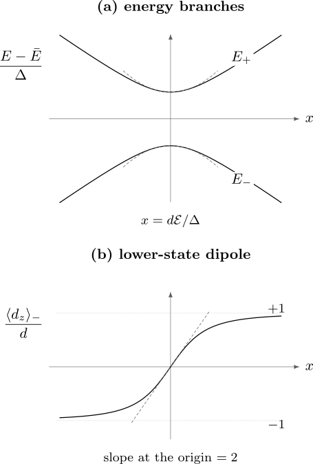
With $x=d\mathcal E/\Delta$, the exact energy branches are even in field and approach linear asymptotes only after strong mixing. Dashed curves show the quadratic and linear weak-field approximations. The lower-state dipole is odd in field: its initial slope is the polarizability, while the exact two-state response saturates at $\lvert d\rvert$.

The Degenerate Warning

Setting $\Delta=0$ before expanding changes the problem qualitatively. The projected Hamiltonian becomes

$$H_2(\mathcal E) = E_0 I - \mathcal E \begin{pmatrix} 0 & d\\ d^* & 0 \end{pmatrix}.$$

Its ordered eigenvalues are

$$E_\pm = E_0 \pm \lvert d\mathcal E\rvert.$$

Equivalently, diagonalize $d_z$ inside the degenerate subspace. Its eigenstates have dipoles $\pm\lvert d\rvert$ and analytic energies

$$E_{p}(\mathcal E) = E_0-p\mathcal E, \qquad p=\pm\lvert d\rvert.$$

The absolute value in the ordered spectrum comes from relabeling the lower and upper branches when the field reverses. Each dipole-labeled branch is linear.

The weak-field and degenerate limits do not commute:

$$\begin{aligned} \mathcal E\to0 \quad\text{at fixed }\Delta\gt0 &: \quad \delta E \propto \mathcal E^2, \\ \Delta\to0 \quad\text{at fixed }\mathcal E\ne0 &: \quad \delta E \propto \lvert\mathcal E\rvert. \end{aligned}$$

The divergent expression $2\lvert d\rvert^2/\Delta$ is not an infinite physical polarizability at exact degeneracy. It is a warning that the nondegenerate Taylor expansion has lost its domain of validity.

For small but nonzero $\Delta$, the response is always quadratic sufficiently close to $\mathcal E=0$, then crosses toward a linear form when

$$\lvert d\mathcal E\rvert \gg \Delta.$$

That crossover is physically useful only if the same field remains weak enough not to mix important states outside the retained pair.

Testing the Two-State Truncation

Let $P$ project onto $\{\lvert g\rangle,\lvert e\rangle\}$ and $Q=I-P$. Exact diagonalization of $PHP$ does not account for $PHQ$ or $QHP$.

At weak field, the full ground-state polarizability is

$$\begin{aligned} \alpha_g ={}& \frac{ 2\lvert d\rvert^2 }{ \Delta } \\ & + 2 \sum_{n\notin\{g,e\}} \frac{ \left| \langle n\vert d_z\vert g\rangle \right|^2 }{ E_n-E_g }. \end{aligned}$$

If $\lvert g\rangle$ is the nondegenerate ground state, every omitted term is nonnegative. The two-state value is then a lower bound on the exact static polarizability, provided the states and matrix elements are exact. For an excited reference state, denominators can have either sign and no such monotonic statement follows.

A practical two-state model should pass two separate tests:

1. Dominant-response test. The retained partner should dominate the sum over states for the observable being calculated.
2. Leakage test. For each important omitted state $\lvert n\rangle$, the ratio

$$\epsilon_n \sim \frac{ \left| \mathcal E \langle n\vert d_z\vert\psi_P\rangle \right| }{ \left| E_n-E_{\psi_P} \right| }$$

should remain small over the stated field range.

Here $\lvert\psi_P\rangle$ is the relevant field-mixed state inside $P$. Near the pair’s internal crossover, it is generally not enough to test leakage from only one bare state.

The desired scale hierarchy for a clean linear-like crossover is

$$\Delta \ll \lvert d\mathcal E\rvert \ll \Delta_{\mathrm{out}},$$

where the second comparison is schematic: $\Delta_{\mathrm{out}}$ must be divided by the appropriate transition-dipole ratio for every omitted channel. A narrow doublet well separated from all other states can realize this hierarchy; a crowded spectrum may not.

What Changes with Permanent Dipoles?

If inversion symmetry is absent, the projected dipole can have diagonal elements:

$$D_2 = \begin{pmatrix} d_g & d\\ d^* & d_e \end{pmatrix}.$$

Then

$$H_2(\mathcal E) = \begin{pmatrix} E_g-\mathcal E d_g & -\mathcal E d\\ -\mathcal E d^* & E_e-\mathcal E d_e \end{pmatrix}.$$

The common dipole $(d_g+d_e)/2$ shifts the trace linearly, while the dipole difference changes the effective detuning. An isolated state can then have a first-order Stark shift without any degeneracy. The symmetric formulas derived above should not be applied after silently setting $d_g$ and $d_e$ to zero.

Validation Ledger

The result passes several checks that probe different parts of the calculation.

Check	Consequence
Hermiticity	energies depend on $\lvert d\rvert^2$, not on the phase of $d$
zero field	$E_-\to E_g$ and $E_+\to E_e$
fixed trace	$\delta E_g+\delta E_e=0$
parity	isolated branches are even in $\mathcal E$
level repulsion	the lower level moves down and the upper level moves up
Hellmann–Feynman	$-\partial E_\pm/\partial\mathcal E$ matches the dipole expectation value
weak field	exact energies reproduce second-order perturbation theory
exact degeneracy	projected diagonalization gives linear dipole-labeled branches
dimensions	$\lvert d\rvert^2\mathcal E^2/\Delta$ has units of energy

These checks validate the projected calculation. Only a convergence study under enlargement of the model space can validate the two-state truncation itself.

Common Mistakes

• Calling $\mathcal E$ small without comparing $\lvert d\mathcal E\rvert$ with $\Delta$.
• Applying the quadratic formula when $\Delta=0$ and interpreting its divergence literally.
• Forgetting the factor $1/2$ in $\delta E=-\alpha\mathcal E^2/2$ for an induced dipole.
• Assigning a positive polarizability to the upper state merely because $\lvert d\rvert^2$ is positive.
• Dropping the complex conjugate in the projected Hamiltonian.
• Treating exact diagonalization of $PHP$ as an exact solution of the full Hilbert-space problem.
• Assuming strong mixing within the pair guarantees negligible leakage to other states.
• Using a static polarizability formula for an oscillating or near-resonant field.
• Confusing a level shift with the shift of a measured transition frequency.

Exercises

1. Derive the exact branches

Starting from $H_2-\bar E I$, derive the characteristic polynomial and the exact energies. Use the trace to prove that the two shifts relative to the bare levels are equal and opposite.

Solution

For $\lambda=E-\bar E$,

$$\begin{aligned} 0 &= \det \begin{pmatrix} -\Delta/2-\lambda & -\mathcal E d\\ -\mathcal E d^* & \Delta/2-\lambda \end{pmatrix} \\ &= \lambda^2 - \frac{\Delta^2}{4} - \lvert d\rvert^2\mathcal E^2. \end{aligned}$$

Thus

$$\lambda_\pm = \pm \sqrt{ \frac{\Delta^2}{4} + \lvert d\rvert^2\mathcal E^2 },$$

which gives the stated $E_\pm$. Because

$$E_-+E_+ = 2\bar E = E_g+E_e,$$

one has

$$(E_--E_g)+(E_+-E_e)=0.$$

Therefore $\delta E_e=-\delta E_g$.

2. Prove the perturbative error formula

Let

$$f = \frac{ \sqrt{1+4\eta^2}-1 }{2}.$$

Show that the relative error of the quadratic lower-state shift is exactly $f$. Find the largest $\eta$ allowed by a two-percent error tolerance.

Solution

From

$$\sqrt{1+4\eta^2}=1+2f,$$

squaring gives

$$\eta^2=f+f^2=f(1+f).$$

The exact shift is $-\Delta f$, while the quadratic result is $-\Delta\eta^2$. Their relative difference is

$$\frac{\eta^2-f}{f} = f.$$

For tolerance $\tau=0.02$,

$$\eta \le \sqrt{\tau(1+\tau)} = \sqrt{0.0204} \approx 0.1428.$$

3. Compute the dipole directly

Assume $d$ is real. Use the mixed lower state to calculate $\langle-\vert d_z\vert-\rangle$ and show that it agrees with the energy derivative.

Solution

Inside the retained subspace,

$$d_z = d \left( \lvert g\rangle\langle e\rvert + \lvert e\rangle\langle g\rvert \right).$$

For

$$\lvert-\rangle = \cos\theta\,\lvert g\rangle + \sin\theta\,\lvert e\rangle,$$

the expectation value is

$$\langle-\vert d_z\vert-\rangle = 2d\sin\theta\cos\theta = d\sin(2\theta).$$

Since

$$\sin(2\theta) = \frac{ 2d\mathcal E }{ \sqrt{ \Delta^2+4d^2\mathcal E^2 } },$$

one obtains

$$\langle-\vert d_z\vert-\rangle = \frac{ d^2\mathcal E }{ \sqrt{ \Delta^2/4+d^2\mathcal E^2 } },$$

which equals $-\partial E_-/\partial\mathcal E$.

4. Explain the singular limit

Why can the finite-gap energy be even in $\mathcal E$ while an exactly degenerate pair has linear Stark branches? Evaluate the limits in both orders.

Solution

At fixed $\Delta\gt0$, each eigenvalue is isolated near zero field and has the expansion

$$\delta E_g = - \frac{ \lvert d\rvert^2\mathcal E^2 }{ \Delta } + O(\mathcal E^4).$$

It is even in field. Sending $\mathcal E\to0$ first therefore gives zero slope.

At $\Delta=0$, the dipole operator must first be diagonalized inside the degenerate subspace. The dipole-labeled states have

$$E_p(\mathcal E)=E_0-p\mathcal E,$$

so their slopes are $\mp\lvert d\rvert$. Inversion exchanges the two branches under field reversal; it does not require each branch to be even.

Thus the expansion at fixed nonzero gap is not uniform as $\Delta\to0$. The two limits select different zeroth-order eigenstates.

5. Audit an omitted state

Add one omitted state $\lvert r\rangle$ above $\lvert g\rangle$, with gap $\Delta_r=E_r-E_g$ and dipole $d_r=\langle r\vert d_z\vert g\rangle$. What fraction of the ground-state polarizability is missed by the two-state model? State a field-level leakage test.

Solution

The retained and omitted contributions are

$$\alpha_g^{(2)} = \frac{2\lvert d\rvert^2}{\Delta}, \qquad \delta\alpha_r = \frac{2\lvert d_r\rvert^2}{\Delta_r}.$$

If these are the only contributions, the missed fraction of the exact polarizability is

$$\frac{ \delta\alpha_r }{ \alpha_g^{(2)}+\delta\alpha_r } = \frac{ \lvert d_r\rvert^2/\Delta_r }{ \lvert d\rvert^2/\Delta + \lvert d_r\rvert^2/\Delta_r }.$$

At finite field, a necessary weak-leakage condition from the bare ground state is

$$\frac{ \lvert d_r\mathcal E\rvert }{ \Delta_r } \ll1.$$

Near strong mixing of the retained pair, one should repeat the test with the actual field-mixed state because it also contains an $\lvert e\rangle$ component.

Cross-Links

• Stark Effect in Atoms
• Worked Problems and Model Calculations
• Stark Effect as a Perturbation Example
• Two-State Hamiltonians
• Second-Order Energy Corrections
• Degenerate Perturbation Theory
• Quasi-Degenerate Perturbation Theory
• Hellmann–Feynman Theorem
• Parity as Inversion
• Stark Effect

References

• J. J. Sakurai and J. Napolitano, Modern Quantum Mechanics, 3rd ed., Cambridge University Press, 2020.
• C. Cohen-Tannoudji, B. Diu, and F. Laloë, Quantum Mechanics, Vol. II, Wiley, 1977.
• L. D. Landau and E. M. Lifshitz, Quantum Mechanics: Non-Relativistic Theory, 3rd ed., Pergamon, 1977.
• C. J. Foot, Atomic Physics, Oxford University Press, 2005.
• J. Mitroy, M. S. Safronova, and C. W. Clark, “Theory and applications of atomic and ionic polarizabilities,” Journal of Physics B 43, 202001 (2010), doi:10.1088/0953-4075/43/20/202001.