Quasi-Degenerate Perturbation Theory

Quasi-degenerate perturbation theory treats several nearby states as one model space. Their small internal splittings and mutual couplings are diagonalized together, while coupling to well-separated states is expanded perturbatively.

The method is needed when levels are not exactly degenerate, yet their detuning is comparable to the perturbation that mixes them. A one-state formula then produces large denominators and predicts large state corrections. Exact diagonalization of the nearby cluster removes those artificial singularities.

The central rule is:

Retain every strongly mixed nearby state in $P$, diagonalize within $P$, and perturb only the coupling between $P$ and $Q$.

Here $P$ projects onto the retained model space and $Q=I-P$ onto its complement. The method interpolates between Nondegenerate Perturbation Theory when $P$ is one-dimensional and Degenerate Perturbation Theory when the unperturbed levels inside $P$ coincide exactly.

The Near-Degeneracy Problem

Suppose two unperturbed states satisfy

$$H_0\lvert a\rangle =E_a^{(0)}\lvert a\rangle, \qquad H_0\lvert b\rangle =E_b^{(0)}\lvert b\rangle,$$

and are coupled by $V_{ab}=\langle a\rvert V\lvert b\rangle$. Nondegenerate perturbation theory tries to assign the mixing amplitude

$$c_{b\leftarrow a}^{(1)} = \lambda \frac{V_{ba}} {E_a^{(0)}-E_b^{(0)}}.$$

This is small only if

$$\lvert\lambda V_{ba}\rvert \ll \left|E_a^{(0)}-E_b^{(0)}\right|.$$

When the two scales are comparable, the exact eigenvectors are order-$1$ mixtures of $\lvert a\rangle$ and $\lvert b\rangle$. No higher-order correction to a state that remains “mostly $a$” can repair a zeroth-order labeling that has already failed.

Near-degeneracy is therefore a power-counting statement, not merely visual closeness on an energy plot. A small spacing matters when an allowed matrix element is large enough to compete with it. Symmetry can make $V_{ab}=0$, in which case nearby levels may cross without mixing.

The Two-State Cure

Retain both states and diagonalize their projected Hamiltonian. Write

$$H_P(\lambda) = \begin{pmatrix} \varepsilon_1(\lambda) & w(\lambda) \\ w^*(\lambda) & \varepsilon_2(\lambda) \end{pmatrix},$$

where the diagonal entries may already include perturbative shifts from remote states. Define

$$\begin{aligned} \bar\varepsilon &= \frac{\varepsilon_1+\varepsilon_2}{2}, \\ d &= \frac{\varepsilon_1-\varepsilon_2}{2}. \end{aligned}$$

The two eigenvalues are

$$E_\pm = \bar\varepsilon \pm \sqrt{d^2+\lvert w\rvert^2}.$$

At zero detuning, $d=0$, the gap is

$$E_+-E_- = 2\lvert w\rvert.$$

The eigenstates are equal-weight mixtures there. Away from the crossing, write $w=\lvert w\rvert e^{i\phi}$ and choose a mixing angle satisfying

$$\tan(2\theta) = \frac{2\lvert w\rvert} {\varepsilon_1-\varepsilon_2}.$$

The phase $\phi$ fixes the relative phase of the two basis components. The detailed eigenvector conventions and Bloch-sphere interpretation belong to Two-State Hamiltonians.

If $\varepsilon_1\gt\varepsilon_2$ and $\lvert w\rvert$ is small compared with their difference, define $\Delta_\varepsilon=\varepsilon_1-\varepsilon_2$. Expansion of the exact roots gives

$$\begin{aligned} E_+ &= \varepsilon_1 + \frac{\lvert w\rvert^2} {\Delta_\varepsilon} \\ &\quad+ O\!\left( \frac{\lvert w\rvert^4}{\Delta_\varepsilon^3} \right), \\ E_- &= \varepsilon_2 - \frac{\lvert w\rvert^2} {\Delta_\varepsilon} \\ &\quad+ O\!\left( \frac{\lvert w\rvert^4}{\Delta_\varepsilon^3} \right). \end{aligned}$$

Thus ordinary second-order level repulsion is the far-detuned expansion of an avoided crossing. The exact square root, rather than a divergent inverse detuning, is the uniform local description.

Model Space and Complement

Let the model space be spanned by $d$ orthonormal unperturbed states,

$$P = \sum_{a=1}^{d} \lvert a\rangle\langle a\rvert, \qquad Q=I-P.$$

Block the Hamiltonian as

$$H = \begin{pmatrix} PHP & PHQ \\ QHP & QHQ \end{pmatrix}.$$

The internal block $PHP$ is not expanded into separate one-state answers. It is diagonalized as a matrix. Remote states influence it through induced diagonal shifts and induced off-diagonal couplings.

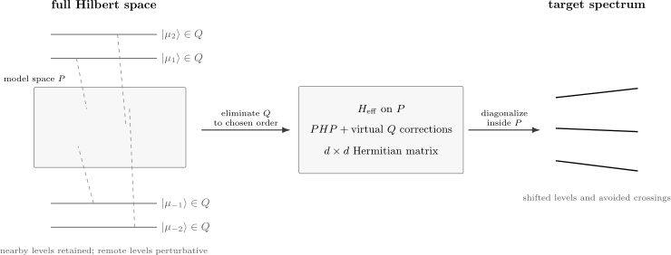
The model space $P$ contains the close levels and all strong internal mixing. Remote $Q$ states are eliminated perturbatively, producing an effective Hamiltonian on $P$. The final diagonalization is exact within that retained space.

For a cluster with unperturbed width

$$W_P = \max_{a\in P}E_a^{(0)} - \min_{a\in P}E_a^{(0)},$$

and distance to the complementary spectrum

$$G_{PQ} = \operatorname{dist} \left( \operatorname{spec}(PH_0P), \operatorname{spec}(QH_0Q) \right),$$

the useful regime is schematically

$$\begin{aligned} W_P &\lesssim \lvert\lambda\rvert\lVert PVP\rVert, \\ \eta_{PQ} &\equiv \frac{ \lvert\lambda\rvert\lVert PVQ\rVert }{G_{PQ}} \ll1. \end{aligned}$$

The first relation says internal mixing must be treated nonperturbatively. The second says elimination of $Q$ remains controlled. For unbounded operators, these norm expressions are only a finite-model diagnostic; domain and relative-boundedness hypotheses require separate analysis.

Exact Energy-Dependent Effective Equation

Project an exact eigenstate as

$$\lvert\Psi\rangle = \lvert\Psi_P\rangle + \lvert\Psi_Q\rangle.$$

If $E-QHQ$ is invertible, the $Q$ equation gives

$$\lvert\Psi_Q\rangle = \frac{1}{E-QHQ} QHP\lvert\Psi_P\rangle.$$

Substitution into the $P$ equation yields

$$H_{\mathrm{eff}}(E) \lvert\Psi_P\rangle = E\lvert\Psi_P\rangle,$$

with

$$\begin{aligned} H_{\mathrm{eff}}(E) &= PHP+\Sigma_P(E), \\ \Sigma_P(E) &= PHQ \frac{1}{E-QHQ} QHP. \end{aligned}$$

This identity is exact where the resolvent exists. Its energy dependence makes the eigenvalue problem nonlinear, and poles signal that a supposedly eliminated state is dynamically relevant. The block derivation, Schur complement, state reconstruction, and normalization belong to Projection Methods. Continuum continuation and resonance interpretation belong to Feshbach Projection Formalism. The one-state energy-dependent expansion belongs to Brillouin–Wigner Perturbation Theory. The Q-box derivative construction of one energy-independent operator for several selected states belongs to Folded Effective Hamiltonians.

Quasi-degenerate perturbation theory expands this exact structure in the coupling to $Q$ while preserving matrix diagonalization inside $P$.

Hermitian Effective Hamiltonian Through Second Order

Let

$$H=H_0+\lambda V,$$

and choose $P$ from eigenstates $\lvert a\rangle$ of $H_0$ with nearby, not necessarily equal, energies $E_a^{(0)}$. Let Greek indices $\mu$ label $Q$ states, and define

$$D_{a\mu} \equiv \frac{1}{E_a^{(0)}-E_\mu^{(0)}}.$$

A standard Hermitian energy-independent effective Hamiltonian through second order has matrix elements

$$\begin{aligned} \bigl(H_{\mathrm{eff}}\bigr)_{ab} ={}& E_a^{(0)}\delta_{ab} +\lambda V_{ab} \\ &+ \lambda^2 \bigl(H_{\mathrm{eff}}^{(2)}\bigr)_{ab} +O(\lambda^3). \end{aligned}$$

Here

$$\bigl(H_{\mathrm{eff}}^{(2)}\bigr)_{ab} = \frac12 \sum_{\mu\in Q} V_{a\mu}V_{\mu b} \bigl(D_{a\mu}+D_{b\mu}\bigr).$$

This is often called a canonical Van Vleck or Löwdin effective Hamiltonian. It is Hermitian because the two denominators are symmetrized between the bra and ket states.

For $a=b$, the second-order term reduces to

$$\bigl(H_{\mathrm{eff}}^{(2)}\bigr)_{aa} = \sum_{\mu\in Q} \frac{\lvert V_{a\mu}\rvert^2} {E_a^{(0)}-E_\mu^{(0)}}.$$

This is the usual second-order energy correction, but the sum excludes the other model-space states. Their effects are generated by diagonalizing $H_{\mathrm{eff}}$ and must not be added again with small denominators.

For $a\ne b$, this same matrix element can be nonzero even when $V_{ab}=0$. Virtual excursions into the eliminated space can therefore shift levels, open or modify avoided-crossing gaps, and generate interactions absent in the directly projected block.

Different effective-Hamiltonian conventions can differ in their off-shell matrix elements. Bloch, canonical Van Vleck, Löwdin, and Schrieffer–Wolff constructions impose different normalization or block-diagonalization choices. When carried out consistently, they reproduce the target exact eigenvalues through the claimed order; some forms are manifestly Hermitian and others are not. Do not combine matrix elements from different conventions term by term.

Exactly Degenerate Limit

If all model-space states have the same unperturbed energy $E_0$, the second-order matrix simplifies to

$$\begin{aligned} \bigl(H_{\mathrm{eff}}\bigr)_{ab} ={}& E_0\delta_{ab} +\lambda V_{ab} \\ &+ \lambda^2 \sum_{\mu\in Q} \frac{V_{a\mu}V_{\mu b}} {E_0-E_\mu^{(0)}} +O(\lambda^3). \end{aligned}$$

At first order, this is precisely the instruction to diagonalize $PVP$. At second order, virtual $Q$ states add another Hermitian matrix that may split any degeneracy left by $PVP$.

Quasi-degenerate theory therefore does not compete with degenerate perturbation theory. It extends the same model-space logic to clusters whose internal splittings are small but nonzero.

Relation to Other Methods

Nondegenerate perturbation theory

Choose $P=\lvert n^{(0)}\rangle\langle n^{(0)}\rvert$. The effective Hamiltonian is a scalar and its second-order term becomes the familiar sum over all $Q$ states.

Degenerate perturbation theory

Set $PH_0P=E_0P$. Diagonalize $PVP$ at first order, followed by induced higher-order matrices if needed.

Brillouin–Wigner and Feshbach methods

Keep $E$ in the $Q$-space resolvent. This retains exact energy dependence but creates a nonlinear eigenvalue problem and a root-selection task.

Folded effective Hamiltonians

Expand the Q-box around a model-space starting energy and resum its energy feedback into one energy-independent interaction. This is useful when several target states should come from one diagonalization, but it introduces Q-box poles, iteration choices, and induced many-body terms. The construction belongs to Folded Effective Hamiltonians.

Schrieffer–Wolff transformation

Construct a perturbative unitary transformation that block-diagonalizes $P$ and $Q$. The resulting energy-independent Hermitian Hamiltonian is especially useful when one wants effective operators as well as energies. Its generator and commutator expansion belong to Schrieffer–Wolff Transformation.

Direct diagonalization

If a converged finite matrix for the full relevant Hilbert space is affordable, Matrix Diagonalization may be simpler and more reliable. The model-space calculation remains valuable for interpretation, parameter dependence, and uncertainty diagnosis.

Choosing the Model Space

A useful $P$ space is large enough to remove every dangerous denominator and small enough that eliminating $Q$ is worthwhile.

Use the following tests:

1. Energy-window test. Include levels whose unperturbed detuning from the target cluster is comparable to retained direct or induced couplings.
2. Matrix-element test. A nearby state with a symmetry-forbidden coupling need not be included for that perturbation, though another allowed interaction may change the conclusion.
3. Stability test. Enlarge $P$ and verify that target eigenvalues and observables change only beyond the claimed order.
4. Symmetry test. Build $P$ from complete symmetry multiplets when the perturbation preserves that symmetry. Cutting a multiplet can create basis-dependent results.
5. Intruder-state test. Monitor the smallest $P$–$Q$ denominator. If a $Q$ level approaches the cluster, promote it into $P$.
6. State-character test. Track eigenvectors by overlaps or symmetry labels rather than sorting eigenvalues independently at each parameter value.

There is no universal energy cutoff. The correct model space depends on both detunings and couplings.

Reconstructing States and Observables

An eigenvector of $H_{\mathrm{eff}}$ supplies only the model-space component. To leading order in the eliminated coupling,

$$\lvert\Psi_Q\rangle \approx \frac{1}{E^{(0)}-QH_0Q} QVP\lvert\Psi_P\rangle.$$

The leakage probability is therefore schematically

$$p_Q = \langle\Psi_Q\vert\Psi_Q\rangle = O(\eta_{PQ}^{,2}).$$

Normalization, transition matrix elements, and expectation values require this dressing. An effective observable generally differs from the bare projection $PAP$ because the same transformation that removes $P$–$Q$ coupling also dresses operators. Using a corrected Hamiltonian with undressed observables can lose terms of the very order one intended to retain.

For an energy-dependent Feshbach Hamiltonian, the derivative of the self-energy also enters normalization. For an energy-independent unitary construction, transform both states and operators with the same unitary map.

Applications

Biased double wells

Localized states $\lvert L\rangle$ and $\lvert R\rangle$ form a two-dimensional model space. Bias supplies the detuning and tunneling supplies the off-diagonal coupling. Diagonalizing the pair gives the avoided crossing. The detailed spatial construction belongs to Coupled Wells and Avoided Crossings.

The tunneling amplitude itself may be exponentially small in a semiclassical parameter. Finite-order power-series perturbation theory need not generate that nonperturbative scale; quasi-degenerate theory organizes the mixing once the amplitude has been calculated or matched.

Atomic and molecular level crossings

External electric or magnetic fields can tune two levels close together. Selection rules determine whether the crossing is exact or avoided. Remote levels contribute Stark, Zeeman, and spin–orbit shifts to the effective matrix, while the nearby pair or multiplet is diagonalized together. This is the setting in which smooth adiabatic potential curves and reliable state tracking matter more than assigning a fixed unperturbed label.

Two-level atoms and dressed-state truncations

For a static two-level approximation, the retained pair must be separated from all other atomic levels by gaps large compared with the relevant couplings. Near resonant driving, the quasi-degenerate pair often lives in a rotating or Floquet representation rather than the bare atomic spectrum. The dynamics and drive-dependent approximations then belong to the time-dependent and Floquet chapters.

Band-crossing preview

Near a crossing momentum $\mathbf k_0$, retain the few bands whose energies coincide or nearly coincide and eliminate remote bands. A two-band effective Hamiltonian often has the form

$$\begin{aligned} H_{\mathrm{eff}}(\mathbf q) &= d_0(\mathbf q)I + \mathbf d(\mathbf q)\cdot\boldsymbol\sigma, \\ \mathbf q &= \mathbf k-\mathbf k_0. \end{aligned}$$

Symmetry may force components of $\mathbf d$ to vanish and protect a crossing. An allowed constant component can open a gap. This is only a preview: crystalline symmetry, topology, and multiband $\mathbf k\cdot\mathbf p$ theory require their own conventions and canonical pages.

Practical Workflow

1. Identify the target energy cluster and all conserved quantum numbers.
2. Estimate detuning-to-coupling ratios for states near the cluster.
3. Put every strongly mixed state in $P$; set $Q=I-P$.
4. Construct $PHP$ and diagonalize it exactly as a first diagnostic.
5. Add the desired order of $Q$-induced shifts and couplings using one consistent effective-Hamiltonian convention.
6. Diagonalize the resulting $H_{\mathrm{eff}}$ without re-expanding its small internal eigenvalue gaps.
7. Reconstruct $Q$-space dressing when states or observables are needed.
8. Enlarge $P$, enlarge the numerical basis, and compare with direct diagonalization where possible.
9. Track branches by overlap and symmetry through avoided crossings.
10. State the perturbative order, model-space definition, and error diagnostic with the result.

Failure Modes

• Leaving one strongly coupled near state in $Q$, producing an intruder denominator.
• Treating the eigenvalues of $H_{\mathrm{eff}}$ as another series in the internal detuning and recreating the original singularity.
• Double counting model-space mixing in both matrix diagonalization and sum-over-states terms.
• Using an unsymmetrized effective Hamiltonian while assuming it is Hermitian.
• Combining a Bloch wave operator with a canonical Van Vleck normalization formula.
• Choosing $P$ by energy alone and ignoring selection rules or large matrix elements.
• Truncating part of a symmetry multiplet.
• Forgetting that approximate localized or valence states may be nonorthogonal.
• Ignoring $Q$-space dressing when computing observables.
• Following sorted eigenvalue indices instead of continuous eigenstate branches.
• Applying a bound-state effective Hamiltonian at a continuum threshold without the correct analytic continuation.
• Assuming that a small avoided-crossing gap is necessarily perturbative; it may be exponentially generated.

Exercises

1. Uniform two-level result

Let

$$H = \begin{pmatrix} \delta/2 & g \\ g^* & -\delta/2 \end{pmatrix}.$$

Find the eigenvalues, the minimum gap as $\delta$ is varied, and the far-detuned expansion.

Solution

The characteristic equation is

$$E^2 = \frac{\delta^2}{4} +\lvert g\rvert^2,$$

so

$$E_\pm = \pm \sqrt{ \frac{\delta^2}{4} +\lvert g\rvert^2 }.$$

The gap is

$$E_+-E_- = 2\sqrt{ \frac{\delta^2}{4} +\lvert g\rvert^2 },$$

whose minimum at $\delta=0$ is $2\lvert g\rvert$. For $\delta\gt0$ and $\lvert g\rvert\ll\delta$,

$$\begin{aligned} E_+ &= \frac{\delta}{2} + \frac{\lvert g\rvert^2}{\delta} + O\!\left( \frac{\lvert g\rvert^4}{\delta^3} \right), \\ E_- &= -\frac{\delta}{2} - \frac{\lvert g\rvert^2}{\delta} + O\!\left( \frac{\lvert g\rvert^4}{\delta^3} \right). \end{aligned}$$

The inverse detuning is valid only in the far-detuned regime; the square root remains finite through the crossing.

2. Remote-state-mediated coupling

Let $P$ contain $\lvert1\rangle$ and $\lvert2\rangle$, and let $Q$ contain one state $\lvert3\rangle$. Assume $V_{12}=0$, but $V_{13}=g_1$ and $V_{32}=g_2$. Find the induced off-diagonal matrix element through second order.

Solution

The Hermitian second-order formula gives

$$\begin{aligned} \bigl(H_{\mathrm{eff}}^{(2)}\bigr)_{12} = \frac{g_1g_2}{2} \Biggl[ &\frac{1}{E_1^{(0)}-E_3^{(0)}} \\ &+ \frac{1}{E_2^{(0)}-E_3^{(0)}} \Biggr]. \end{aligned}$$

The physical contribution to the Hamiltonian is $\lambda^2(H_{\mathrm{eff}}^{(2)})_{12}$. Even though there is no direct coupling, the path $1\to3\to2$ mediates mixing. Hermiticity gives the reverse element as its complex conjugate.

3. Degenerate limit

Take $E_1^{(0)}=E_2^{(0)}=E_0$ in Exercise 2. Show how the symmetrized denominator simplifies.

Solution

Both denominators become $E_0-E_3^{(0)}$, so

$$\bigl(H_{\mathrm{eff}}^{(2)}\bigr)_{12} = \frac{g_1g_2} {E_0-E_3^{(0)}}.$$

The factor $1/2$ is canceled by the two equal terms. This is the usual second-order effective matrix within an exactly degenerate subspace.

4. Choosing a model space

Three unperturbed levels have energies $0$, $0.03\Delta$, and $\Delta$. At the physical coupling, the first two are connected by a matrix element of magnitude $0.05\Delta$, while their couplings to the third have magnitude at most $0.02\Delta$. Which states should be in the first model-space trial?

Solution

The detuning between the first two states is $0.03\Delta$, smaller than their coupling scale $0.05\Delta$. They must be retained and diagonalized together. The third state is separated by a gap of order $\Delta$, while its coupling is at most $0.02\Delta$, giving a mixing ratio of order $0.02$. It is a reasonable first $Q$-space state.

This is a starting choice, not a proof. One should add the third state to $P$ as a stability check and verify that target quantities change only beyond the intended order.

5. Leading leakage probability

Let $\lvert\Psi_P\rangle$ be normalized inside $P$. Using the leading reconstruction formula, write the $Q$-space probability in the $H_0$ eigenbasis.

Solution

Let $c_a=\langle a\vert\Psi_P\rangle$ and let $\lvert\mu\rangle$ label $Q$ states. To first order,

$$\langle\mu\vert\Psi_Q\rangle \approx \lambda \frac{ \sum_{a\in P}V_{\mu a}c_a }{ E^{(0)}-E_\mu^{(0)} }.$$

Therefore

$$p_Q \approx \lambda^2 \sum_{\mu\in Q} \frac{ \left| \sum_{a\in P}V_{\mu a}c_a \right|^2 }{ \left(E^{(0)}-E_\mu^{(0)}\right)^2 }.$$

Interference between amplitudes from different model-space components is physical and can enhance or suppress leakage.

6. Biased double well

For

$$H_{LR} = \begin{pmatrix} \epsilon & -K \\ -K & -\epsilon \end{pmatrix},$$

find the energies and state character in the limits $\lvert\epsilon\rvert\gg K$ and $\epsilon=0$.

Solution

The energies are

$$E_\pm = \pm\sqrt{\epsilon^2+K^2}.$$

For $\lvert\epsilon\rvert\gg K$, each eigenstate is predominantly localized in one well and receives a small admixture of the other. At $\epsilon=0$, the eigenstates are the symmetric and antisymmetric combinations

$$\frac{ \lvert L\rangle\pm\lvert R\rangle }{\sqrt2},$$

with a splitting $2K$. The exact two-state result is uniform across the bias value where a one-state expansion would fail.

Cross-Links

• Time-Independent Perturbation Theory for method selection and notation.
• Degenerate Perturbation Theory for exact unperturbed multiplets.
• Higher-Order Structure for one-state recursion, analytic structure, and stopping rules.
• Brillouin–Wigner Perturbation Theory for energy-dependent denominators.
• Rayleigh–Schrödinger Perturbation Theory for the energy-independent order expansion and its normalization conventions.
• Stark Effect as a Perturbation Example for a physical two-state crossover controlled by an electric-field matrix element.
• Projection Methods for exact P/Q elimination, reconstruction, and projected normalization.
• Folded Effective Hamiltonians for Q-box derivatives and energy-independent model-space interactions.
• Feshbach Projection Formalism for exact $P$–$Q$ elimination and resonances.
• Schrieffer–Wolff Transformation for unitary block diagonalization and effective operators.
• Two-State Hamiltonians for exact two-dimensional spectra and eigenvectors.
• Coupled Wells and Avoided Crossings for the canonical spatial realization.
• Degeneracy Lifting for symmetry-protected and symmetry-broken splitting.

References

• P.-O. Löwdin, “A Note on the Quantum-Mechanical Perturbation Theory,” Journal of Chemical Physics 19, 1396–1401 (1951), doi:10.1063/1.1748067.
• C. Bloch, “Sur la théorie des perturbations des états liés,” Nuclear Physics 6, 329–347 (1958), doi:10.1016/0029-5582(58)90116-0.
• J. des Cloizeaux, “Extension d’une formule de Lagrange à des problèmes de valeurs propres,” Nuclear Physics 20, 321–346 (1960), doi:10.1016/0029-5582(60)90177-2.
• T. Kato, Perturbation Theory for Linear Operators, 2nd ed., Springer, 1976; reprint 1995, doi:10.1007/978-3-642-66282-9.
• I. Lindgren and J. Morrison, Atomic Many-Body Theory, 2nd ed., Springer, 1986.
• J. R. Schrieffer and P. A. Wolff, “Relation between the Anderson and Kondo Hamiltonians,” Physical Review 149, 491–492 (1966), doi:10.1103/PhysRev.149.491.
• S. Bravyi, D. P. DiVincenzo, and D. Loss, “Schrieffer–Wolff Transformation for Quantum Many-Body Systems,” Annals of Physics 326, 2793–2826 (2011), doi:10.1016/j.aop.2011.06.004.
• A. Messiah, Quantum Mechanics, Vol. II, North-Holland, 1962, Chapter XVII.