First-Order State Corrections

The first-order state correction is the leading change in the eigenvector of an isolated energy level under a weak static perturbation. In intermediate normalization it is

$$\lvert n^{(1)}\rangle = \sum_{m\ne n} \frac{ \langle m^{(0)}\rvert V \lvert n^{(0)}\rangle }{ E_n^{(0)}-E_m^{(0)} } \lvert m^{(0)}\rangle.$$

The physical change is $\lambda\lvert n^{(1)}\rangle$, not $\lvert n^{(1)}\rangle$ by itself. The formula says that a perturbation rotates the reference state toward every state it couples to, with each amplitude suppressed by the corresponding energy separation.

This page owns the interpretation, normalization choices, observable response, symmetry diagnostics, and worked checks associated with that formula. The complete order-by-order derivation remains on Nondegenerate Perturbation Theory.

Result at a Glance

Let

$$\begin{aligned} H(\lambda) &= H_0+\lambda V+O(\lambda^2), \\ H_0\lvert n^{(0)}\rangle &= E_n^{(0)}\lvert n^{(0)}\rangle, \end{aligned}$$

where $E_n^{(0)}$ is a simple isolated eigenvalue and $\lvert n^{(0)}\rangle$ is normalized. Expand the corresponding branch as

$$\lvert n(\lambda)\rangle = \lvert n^{(0)}\rangle + \lambda\lvert n^{(1)}\rangle + O(\lambda^2).$$

Define

$$\begin{aligned} V_{mn} &\equiv \langle m^{(0)}\rvert V \lvert n^{(0)}\rangle, \\ \Delta_{nm} &\equiv E_n^{(0)}-E_m^{(0)}. \end{aligned}$$

With the convention

$$\langle n^{(0)}\vert n(\lambda)\rangle=1,$$

the correction is

$$\lvert n^{(1)}\rangle = \sum_{m\ne n} \frac{V_{mn}}{\Delta_{nm}} \lvert m^{(0)}\rangle.$$

The same result can be written without choosing a complete discrete basis. Introduce

$$\begin{aligned} P_n &= \lvert n^{(0)}\rangle \langle n^{(0)}\rvert, \\ Q_n &= I-P_n, \\ R_n' &= Q_n \frac{1}{E_n^{(0)}-H_0} Q_n. \end{aligned}$$

Then

$$\lvert n^{(1)}\rangle = R_n'V\lvert n^{(0)}\rangle.$$

The inverse in $R_n'$ acts only on the complementary subspace. This is why an exact degeneracy makes the isolated-level formula undefined.

Requirement	What it does
$E_n^{(0)}$ is isolated and nondegenerate	Makes the reduced denominator invertible near the target state
$V$ connects states in the relevant operator domain	Makes the matrix elements and projected equation meaningful
$\lvert\lambda V_{mn}/\Delta_{nm}\rvert$ is small for important channels	Keeps induced mixing perturbative
The chosen eigenvalue branch can be tracked continuously	Prevents relabeling states at an avoided crossing
A normalization and phase convention is stated	Fixes the otherwise arbitrary component parallel to the reference ket

What the Correction Means

The coefficients

$$c_{m\leftarrow n}^{(1)} = \frac{V_{mn}}{\Delta_{nm}}$$

are amplitudes in the unperturbed energy basis. Two independent pieces determine each one:

• $V_{mn}$ asks whether the perturbation can connect the two states and how strongly;
• $\Delta_{nm}^{-1}$ measures how easily that coupling rotates the eigenvector.

A large matrix element does not necessarily imply strong mixing if the gap is much larger. Conversely, a modest matrix element can invalidate nondegenerate perturbation theory when the coupled level is nearby.

For $m\ne n$, an energy measurement in the reference basis has probability

$$\begin{aligned} p_m(\lambda) &= \left| \langle m^{(0)}\vert n(\lambda)\rangle \right|^2 \\ &= \lambda^2 \frac{\lvert V_{mn}\rvert^2} {\lvert\Delta_{nm}\rvert^2} + O(\lambda^3). \end{aligned}$$

The new amplitude is first order, but its probability is second order. This does not mean all observable effects wait until second order. Interference between the reference amplitude and the correction changes many expectation values linearly in $\lambda$.

In a unit-normalized phase convention, the survival probability in the reference ray is

$$\begin{aligned} \left| \langle n^{(0)}\vert n(\lambda)\rangle \right|^2 ={}& 1 - \lambda^2 \sum_{m\ne n} \frac{\lvert V_{mn}\rvert^2} {\lvert\Delta_{nm}\rvert^2} \\ &+ O(\lambda^3). \end{aligned}$$

Thus the norm of the orthogonal first-order correction measures how quickly the perturbed ray leaves the unperturbed one.

The Projection That Produces the Formula

The first-order part of the eigenvalue equation is

$$\bigl(H_0-E_n^{(0)}\bigr) \lvert n^{(1)}\rangle = \bigl(E_n^{(1)}-V\bigr) \lvert n^{(0)}\rangle.$$

For $m\ne n$, projection with $\langle m^{(0)}\rvert$ removes the term proportional to $E_n^{(1)}$ and gives

$$\bigl(E_m^{(0)}-E_n^{(0)}\bigr) \langle m^{(0)}\vert n^{(1)}\rangle = -V_{mn}.$$

Therefore

$$\langle m^{(0)}\vert n^{(1)}\rangle = \frac{V_{mn}} {E_n^{(0)}-E_m^{(0)}}.$$

This determines every component orthogonal to $\lvert n^{(0)}\rangle$. The eigenvalue equation does not determine the parallel component because adding a multiple of $\lvert n^{(0)}\rangle$ changes the representative ket but not its ray to first order. A normalization and phase convention supplies the missing condition.

Projectors Make the Physical Change Explicit

A ket contains an arbitrary global phase. The rank-one spectral projector

$$\Pi_n(\lambda) = \lvert n(\lambda)\rangle \langle n(\lambda)\rvert$$

does not. Its first derivative at $\lambda=0$ is

$$\Pi_n^{(1)} = \lvert n^{(1)}\rangle \langle n^{(0)}\rvert + \lvert n^{(0)}\rangle \langle n^{(1)}\rvert.$$

For a self-adjoint $H_0$ and Hermitian $V$, the reduced-resolvent form is

$$\Pi_n^{(1)} = R_n'VP_n + P_nVR_n'.$$

This operator is independent of a $\lambda$-dependent phase assigned to the eigenket. It is often the cleanest object for response calculations because

$$\left. \frac{d}{d\lambda} \langle A\rangle_n \right|_{\lambda=0} = \operatorname{Tr} \bigl(\Pi_n^{(1)}A\bigr)$$

when $A$ itself is independent of $\lambda$.

The sum-over-states formula is shorthand for the spectral decomposition of $R_n'$. If $H_0$ also has continuum spectrum, the resolution of the identity contains integrals as well as sums. Omitting those continuum contributions can give a finite-looking but incomplete answer.

Energy Denominators and Control

The channel-by-channel mixing parameter is

$$\eta_{mn} = \left| \frac{\lambda V_{mn}} {\Delta_{nm}} \right|.$$

The isolated-level treatment requires $\eta_{mn}\ll1$ for every channel that materially contributes. A collective diagnostic is

$$\begin{aligned} \epsilon_{mathrm{mix}}^2 &\equiv \lambda^2 \langle n^{(1)}\vert n^{(1)}\rangle \\ &= \lambda^2 \sum_{m\ne n} \frac{\lvert V_{mn}\rvert^2} {\lvert\Delta_{nm}\rvert^2}. \end{aligned}$$

The second line assumes a complete discrete orthonormal basis; continuum terms must be included when present. Small $\epsilon_{mathrm{mix}}$ is a useful error indicator, although it is not a universal theorem guaranteeing convergence of the full perturbation series.

If the target eigenvalue is separated from the rest of the spectrum by

$$g_n = \inf_{m\ne n} \lvert E_m^{(0)}-E_n^{(0)}\rvert,$$

then, in a setting where the indicated norms are finite,

$$\lVert \lambda\lvert n^{(1)}\rangle \rVert \le \frac{ \lvert\lambda\rvert \lVert Q_nV\lvert n^{(0)}\rangle\rVert }{g_n}.$$

This bound makes the spectral role of the gap explicit. It can still be conservative, and it says nothing by itself about higher-order analyticity.

Diagnostic	Interpretation	Response
One $\eta_{mn}$ is order one	A nearby state rotates strongly into the target	Diagonalize the coupled subspace
Many individually small terms make $\epsilon_{mathrm{mix}}$ large	Mixing is distributed over many states	Enlarge the basis or use a resolvent calculation
The sum changes strongly with a basis cutoff	High-energy or continuum tails matter	Perform convergence and sum-rule checks
A symmetry-forbidden matrix element appears numerically	Basis or implementation breaks the symmetry	Check quantum numbers and numerical tolerances
The tracked eigenvector swaps identity	The branch passed through an avoided crossing	Track by overlap and use a local subspace model

For systematic guidance on dimensionless ratios and residual estimates, see Small Parameters and Error Estimates.

Normalization and Phase Conventions

The most general first-order solution can be written

$$\lvert n^{(1)}\rangle = \sum_{m\ne n} \frac{V_{mn}}{\Delta_{nm}} \lvert m^{(0)}\rangle + c_n\lvert n^{(0)}\rangle.$$

Unit normalization gives

$$0 = \left. \frac{d}{d\lambda} \langle n(\lambda)\vert n(\lambda)\rangle \right|_{\lambda=0} = 2\operatorname{Re}c_n.$$

It fixes the real part of $c_n$, but not its imaginary part. Under a smooth phase change

$$\lvert n(\lambda)\rangle \longmapsto e^{i\chi(\lambda)} \lvert n(\lambda)\rangle,$$

the coefficient changes as

$$c_n \longmapsto c_n+i\chi'(0).$$

The imaginary part is therefore phase convention, not new physics.

Convention	Condition	Consequence at first order
Intermediate normalization	$\langle n^{(0)}\vert n(\lambda)\rangle=1$	Sets $c_n=0$ and simplifies recursion
Unit norm only	$\langle n(\lambda)\vert n(\lambda)\rangle=1$	Sets $\operatorname{Re}c_n=0$ but leaves phase freedom
Parallel-transport phase	$\langle n(\lambda)\vert\partial_\lambda n(\lambda)\rangle=0$	Removes the local phase component and sets $c_n=0$ at the expansion point

Intermediate normalization is not exact unit normalization. Since $\langle n^{(0)}\vert n^{(1)}\rangle=0$,

$$\left\lVert \lvert n^{(0)}\rangle + \lambda\lvert n^{(1)}\rangle \right\rVert^2 = 1 + \lambda^2 \langle n^{(1)}\vert n^{(1)}\rangle.$$

The truncated vector can be normalized explicitly as

$$\lvert n(\lambda)\rangle_{mathrm{tr}} = \frac{ \lvert n^{(0)}\rangle + \lambda\lvert n^{(1)}\rangle }{ \sqrt{ 1+\lambda^2 \langle n^{(1)}\vert n^{(1)}\rangle } }.$$

This normalization changes no first-order expectation value. At second order, however, the parallel normalization term must be included consistently. The underlying distinction between a ray, a normalized representative, and its remaining global phase is reviewed on Normalization.

Corrections to Expectation Values

Let $A$ be a Hermitian observable independent of $\lambda$. For a normalized state through first order,

$$\begin{aligned} \langle A\rangle_n(\lambda) ={}& \langle n^{(0)}\rvert A \lvert n^{(0)}\rangle \\ &+ 2\lambda\, \operatorname{Re} \langle n^{(0)}\rvert A \lvert n^{(1)}\rangle \\ &+ O(\lambda^2). \end{aligned}$$

In matrix-element form,

$$\begin{aligned} \langle A\rangle_n(\lambda) ={}& A_{nn} \\ &+ 2\lambda\, \operatorname{Re} \sum_{m\ne n} \frac{A_{nm}V_{mn}} {\Delta_{nm}} \\ &+ O(\lambda^2), \end{aligned}$$

where $A_{nm}=\langle n^{(0)}\rvert A\lvert m^{(0)}\rangle$.

If the observable also depends on the parameter,

$$A(\lambda) = A_0+\lambda\dot A_0+O(\lambda^2),$$

then

$$\begin{aligned} \left. \frac{d\langle A\rangle_n}{d\lambda} \right|_{0} ={}& \langle n^{(0)}\rvert \dot A_0 \lvert n^{(0)}\rangle \\ &+ 2\operatorname{Re} \sum_{m\ne n} \frac{(A_0)_{nm}V_{mn}} {\Delta_{nm}}. \end{aligned}$$

The first term is explicit operator response; the second is state response. Omitting either one can give the wrong derivative.

Several quick consequences follow:

• If $A$ commutes with $H_0$ and the reference spectrum is nondegenerate, $A$ is diagonal in that basis, so the state-mixing contribution vanishes at first order.
• A zero first-order energy correction does not imply a zero first-order change in another observable.
• State corrections should be converted into probabilities, expectation values, transition matrix elements, or projector changes before being assigned physical meaning.

For the statistical interpretation of $\langle A\rangle$, see Expectation Values.

Selection Rules Make the Mixing Sparse

Let a unitary symmetry $U$ commute with $H_0$. Suppose

$$\begin{aligned} U\lvert n^{(0)}\rangle &= u_n\lvert n^{(0)}\rangle, \\ U\lvert m^{(0)}\rangle &= u_m\lvert m^{(0)}\rangle, \\ UVU^\dagger &= u_VV. \end{aligned}$$

Then

$$V_{mn} = u_m^*u_Vu_nV_{mn}.$$

A nonzero mixing coefficient therefore requires

$$u_m^*u_Vu_n=1.$$

For parity, if the perturbation has parity $\pi_V$, only states satisfying

$$\pi_m = \pi_V\pi_n$$

can appear in $\lvert n^{(1)}\rangle$. An odd perturbation mixes a parity eigenstate only with states of opposite parity. Consequently:

• its diagonal matrix element vanishes, so the first-order energy shift is zero;
• the state can still change at first order;
• an odd observable can acquire a linear expectation value;
• an even observable has no linear state-response term in a parity eigenstate.

Selection rules eliminate terms exactly within the stated symmetry model. They do not rank the sizes of the allowed terms, and they can weaken when the symmetry is broken. The canonical symmetry treatment is Selection Rules.

Exact Two-Level Check

Consider

$$\begin{aligned} H(\lambda) &= \begin{pmatrix} E_1 & \lambda v \\ \lambda v^* & E_2 \end{pmatrix}, \\ \Delta &\equiv E_2-E_1\gt0. \end{aligned}$$

and write $v=\lvert v\rvert e^{i\phi}$. The exact eigenvalues are

$$E_\pm = \frac{E_1+E_2}{2} \pm \frac{1}{2} \sqrt{ \Delta^2+4\lambda^2\lvert v\rvert^2 }.$$

Choose the mixing angle $0\le\theta\lt\pi/4$ through

$$\tan(2\theta) = \frac{2\lambda\lvert v\rvert}{\Delta}.$$

The lower eigenstate can be written

$$\lvert -\rangle = \cos\theta\lvert1\rangle - e^{-i\phi} \sin\theta\lvert2\rangle.$$

For $\lambda\lvert v\rvert\ll\Delta$,

$$\theta = \frac{\lambda\lvert v\rvert}{\Delta} + O(\lambda^3),$$

so

$$\lvert -\rangle = \lvert1\rangle - \lambda\frac{v^*}{\Delta} \lvert2\rangle + O(\lambda^2).$$

This is exactly the perturbative state correction because

$$\frac{V_{21}}{E_1-E_2} = -\frac{v^*}{\Delta}.$$

The admixture amplitude is order $\lambda$, while the off-diagonal coupling changes the energies only at order $\lambda^2$. Eigenvectors can therefore be more sensitive than eigenvalues.

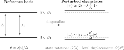
An off-diagonal coupling rotates the eigenvectors by $\theta\simeq\lambda\lvert v\rvert/\Delta$ even when the associated level displacement begins only at order $\lambda^2$.

The probability of finding the lower exact state in $\lvert2\rangle$ is

$$\sin^2\theta = \lambda^2 \frac{\lvert v\rvert^2}{\Delta^2} + O(\lambda^4).$$

When $\lambda\lvert v\rvert$ becomes comparable to $\Delta$, the mixing angle is no longer small. The exact two-state diagonalization remains well behaved, while the nondegenerate expansion has lost its control parameter. At exact degeneracy one must begin with Degenerate Perturbation Theory.

Worked Example: A Linear Force on an Oscillator

Take

$$\begin{aligned} H_0 &= \hbar\omega \left(a^\dagger a+\frac12\right), \\ V &= Fx = F\sqrt{\frac{\hbar}{2m\omega}} \bigl(a+a^\dagger\bigr). \end{aligned}$$

Parity gives $\langle n\rvert x\lvert n\rangle=0$, so the first-order energy correction vanishes. The state does not remain unchanged. Since $x$ connects only adjacent oscillator levels,

$$\begin{aligned} \lvert n^{(1)}\rangle ={}& \varepsilon_F \Bigl( \sqrt n\lvert n-1\rangle \\ &\qquad - \sqrt{n+1}\lvert n+1\rangle \Bigr), \end{aligned}$$

where the dimensionless mixing scale is

$$\varepsilon_F = \frac{F}{\sqrt{2m\hbar\omega^3}}.$$

The signs come from the opposite denominators

$$\begin{aligned} E_n^{(0)}-E_{n-1}^{(0)} &= +\hbar\omega, \\ E_n^{(0)}-E_{n+1}^{(0)} &= -\hbar\omega. \end{aligned}$$

The induced position is

$$\begin{aligned} \langle x\rangle_n(\lambda) &= 2\lambda\, \operatorname{Re} \langle n\rvert x\lvert n^{(1)}\rangle +O(\lambda^2) \\ &= -\frac{\lambda F}{m\omega^2} +O(\lambda^2). \end{aligned}$$

This linear observable response is present even though the linear energy shift is zero.

The model has an exact check. Define the displacement operator

$$D(\alpha) = \exp \bigl( \alpha a^\dagger-\alpha^*a \bigr).$$

Completing the square shows that the exact eigenstate is, up to a phase,

$$\lvert n(\lambda)\rangle = D(-\lambda\varepsilon_F) \lvert n\rangle.$$

Expanding the displacement operator gives

$$\begin{aligned} D(-\lambda\varepsilon_F) ={}& I + \lambda\varepsilon_F \bigl(a-a^\dagger\bigr) \\ &+ O(\lambda^2), \end{aligned}$$

which reproduces the perturbative coefficients. The exact position shift is $-\lambda F/(m\omega^2)$, so the state correction, symmetry argument, dimensions, and observable response all agree. The exact oscillator structure is reviewed on Quantum Harmonic Oscillator.

Geometric Meaning

For a differentiable nondegenerate eigenstate at a general parameter value,

$$H(\lambda)\lvert n(\lambda)\rangle = E_n(\lambda)\lvert n(\lambda)\rangle.$$

Projecting its derivative orthogonally to the state gives the exact local identity

$$\begin{aligned} Q_n\lvert\partial_\lambda n\rangle ={}& \sum_{m\ne n} \frac{ \langle m\rvert \partial_\lambda H \lvert n\rangle }{E_n-E_m} \lvert m\rangle. \end{aligned}$$

At $\lambda=0$ for $\partial_\lambda H=V$, this is the first-order state correction. The orthogonal derivative is phase independent; the omitted parallel derivative is the arbitrary local phase direction.

Its squared norm is the parameter-space quantum metric component

$$\begin{aligned} g_{\lambda\lambda}^{(n)} &= \langle\partial_\lambda n\rvert Q_n \lvert\partial_\lambda n\rangle \\ &= \sum_{m\ne n} \frac{ \left| \langle m\rvert \partial_\lambda H \lvert n\rangle \right|^2 }{(E_n-E_m)^2}. \end{aligned}$$

For nearby normalized states, define the fidelity

$$\begin{aligned} \mathcal F_n(\lambda,\delta\lambda) &\equiv \left| \langle n(\lambda)\vert n(\lambda+\delta\lambda)\rangle \right|^2, \\ \mathcal F_n(\lambda,\delta\lambda) &= 1 - g_{\lambda\lambda}^{(n)} (\delta\lambda)^2 \\ &\quad +O((\delta\lambda)^3). \end{aligned}$$

Thus the same gap-weighted matrix elements that control perturbative mixing also measure local distinguishability of nearby eigenstates. A small gap can make this metric large, but the isolated-level formula itself must be abandoned at an actual degeneracy. The canonical geometric framework is Fubini–Study Geometry.

Computing Without an Explicit State Sum

An explicit sum over eigenstates is often inconvenient or numerically unstable. Instead solve the projected inhomogeneous equation

$$\begin{aligned} \bigl(H_0-E_n^{(0)}\bigr) \lvert\chi_n\rangle ={}& - \bigl(V-E_n^{(1)}\bigr) \lvert n^{(0)}\rangle, \\ \langle n^{(0)}\vert\chi_n\rangle ={}&0. \end{aligned}$$

The solution is $\lvert\chi_n\rangle=\lvert n^{(1)}\rangle$. In coordinate space this becomes an inhomogeneous differential equation; in a finite basis it becomes a constrained linear solve. This approach is closely related to reduced resolvents and Dalgarno–Lewis methods discussed on Sum Rules and Completeness Tricks.

Useful validation checks are:

1. verify $\langle n^{(0)}\vert\chi_n\rangle=0$ in the chosen convention;
2. substitute the result back into the inhomogeneous equation and inspect its residual;
3. test symmetry-forbidden components against zero;
4. enlarge the basis or spatial domain and check convergence;
5. compare with a centered finite difference of exact eigenvectors after aligning their phases;
6. track the eigenvalue branch by overlap, not only by sorted energy index.

For the finite-difference check, phase alignment is essential. Two numerical eigensolvers may return physically identical eigenvectors with unrelated global phases, making an unaligned difference meaningless.

Failure Modes

This isolated-level formula can fail or mislead when:

• an exactly degenerate state appears in the denominator;
• a nearly degenerate state has $\eta_{mn}$ of order one;
• many weak channels accumulate into a large total correction;
• continuum contributions or high-energy tails are omitted;
• the perturbation changes the operator domain or boundary conditions in a singular way;
• an eigenstate branch is relabeled at an avoided crossing;
• an unphysical phase difference is mistaken for a large derivative;
• a truncated ket is used as though it were exactly normalized;
• the observable depends explicitly on $\lambda$ but only state response is included;
• low-order accuracy is mistaken for convergence of the full series.

Exact or near degeneracy is repaired by enlarging the model space and diagonalizing the coupled block. Other failures may require a resolvent treatment, a better basis, direct numerical diagonalization, or a nonperturbative method. See Common Failure Modes for the broader method-selection guide.

Practical Workflow

1. Specify $H_0$, $V$, and the physical meaning and units of $\lambda$.
2. Identify the target eigenvalue and test whether it is isolated on the perturbative scale.
3. Apply symmetry and selection rules before calculating matrix elements.
4. Compute only the allowed $V_{mn}$ and retain the signs of $\Delta_{nm}$.
5. Form $\eta_{mn}$ and $\epsilon_{mathrm{mix}}$ before setting $\lambda=1$.
6. State the normalization and phase convention.
7. Convert the ket correction into the observable, projector, or fidelity quantity of interest.
8. Include explicit parameter dependence of the observable when present.
9. Check dimensions, symmetry, normalization, basis convergence, and an exact or numerical limit.
10. Enlarge the model space whenever a coupled gap is too small.

Common Mistakes

• Calling $\lvert n^{(1)}\rangle$ the physical admixture instead of $\lambda\lvert n^{(1)}\rangle$.
• Including the $m=n$ term in the denominator sum.
• Reversing $E_n^{(0)}-E_m^{(0)}$ and losing the relative signs of components.
• Assuming intermediate normalization means exact unit norm.
• Treating the arbitrary parallel or phase component as observable.
• Squaring the correction and concluding that no quantity changes at first order.
• Ignoring selection rules that make most matrix elements vanish.
• Using the nondegenerate formula for an exact or near degeneracy.
• Forgetting continuum states in a completeness relation.
• Comparing raw numerical eigenvectors without phase alignment.

Exercises

Normalization and phase freedom

Write the first-order correction as

$$\lvert n^{(1)}\rangle = \lvert n_\perp^{(1)}\rangle + c_n\lvert n^{(0)}\rangle,$$

where $\langle n^{(0)}\vert n_\perp^{(1)}\rangle=0$. Show that unit normalization fixes only $\operatorname{Re}c_n$, and explain how a phase choice sets the remaining part to zero.

Solution

Expanding the norm gives

$$\begin{aligned} \langle n(\lambda)\vert n(\lambda)\rangle &= 1 + \lambda(c_n+c_n^*) + O(\lambda^2). \end{aligned}$$

Unit normalization therefore requires

$$c_n+c_n^*=0,$$

or $\operatorname{Re}c_n=0$. The remaining $c_n=i\beta$ is imaginary. Under

$$\lvert n(\lambda)\rangle \longmapsto e^{i\chi(\lambda)} \lvert n(\lambda)\rangle,$$

one has $c_n\mapsto c_n+i\chi'(0)$. Choosing $\chi'(0)=-\beta$ sets $c_n=0$. Intermediate normalization and the local parallel-transport phase both make this choice at the expansion point.

Two-level admixture

For the two-level Hamiltonian in the exact check, compute the first-order correction to $\lvert1\rangle$, the probability of finding $\lvert2\rangle$ in the lower eigenstate through order $\lambda^2$, and the perturbative validity condition.

Solution

Since $V_{21}=v^*$ and $E_1-E_2=-\Delta$,

$$\lvert1^{(1)}\rangle = -\frac{v^*}{\Delta} \lvert2\rangle.$$

Thus

$$\lvert-\rangle = \lvert1\rangle - \lambda\frac{v^*}{\Delta} \lvert2\rangle + O(\lambda^2).$$

The $\lvert2\rangle$ probability is

$$p_2 = \lambda^2 \frac{\lvert v\rvert^2}{\Delta^2} + O(\lambda^4).$$

The expansion is controlled when

$$\frac{\lvert\lambda v\rvert}{\Delta} \ll1.$$

When this ratio is not small, the exact two-state diagonalization is the appropriate organization.

Displaced oscillator response

For $H=H_0+\lambda Fx$, use the first-order state correction to compute $\langle x\rangle_n$ and the leading probability that an energy measurement of $H_0$ finds $n+1$.

Solution

The correction is

$$\begin{aligned} \lvert n^{(1)}\rangle ={}& \varepsilon_F \Bigl( \sqrt n\lvert n-1\rangle \\ &\qquad - \sqrt{n+1}\lvert n+1\rangle \Bigr). \end{aligned}$$

Using $x=x_0(a+a^\dagger)$ with $x_0=\sqrt{\hbar/(2m\omega)}$,

$$\begin{aligned} \langle n\rvert x\lvert n^{(1)}\rangle &= -x_0\varepsilon_F \\ &= -\frac{F}{2m\omega^2}. \end{aligned}$$

Therefore

$$\langle x\rangle_n = -\frac{\lambda F}{m\omega^2} + O(\lambda^2).$$

The $n+1$ amplitude is $-\lambda\varepsilon_F\sqrt{n+1}$, so

$$p_{n+1} = \lambda^2\varepsilon_F^2(n+1) + O(\lambda^3).$$

The expectation value responds at first order because it contains interference with the reference state, whereas the new-basis probability begins at second order.

Parity and linear response

Suppose $H_0$ is parity invariant, $\lvert n^{(0)}\rangle$ has definite parity, and $V$ is odd. Determine the parity of $\lvert n^{(1)}\rangle$. Show that the first-order state contribution to an even observable vanishes, while an odd observable can have a nonzero linear response.

Solution

An odd $V$ connects $\lvert n^{(0)}\rangle$ only to states of opposite parity. Hence every term in $\lvert n^{(1)}\rangle$ has parity opposite to the reference state.

For an even observable $A_+$, the matrix element

$$\langle n^{(0)}\rvert A_+ \lvert n^{(1)}\rangle$$

connects states of opposite parity through an even operator, so it vanishes. The first-order state-response term is therefore zero.

For an odd observable $A_-$, the same bra and ket have the parity relation required for a nonzero matrix element. Symmetry permits

$$2\lambda\operatorname{Re} \langle n^{(0)}\rvert A_- \lvert n^{(1)}\rangle,$$

although its numerical value still depends on the allowed matrix elements.

Phase independence of the projector

Let $\lvert n(\lambda)\rangle$ be normalized and define $\Pi_n(\lambda)=\lvert n(\lambda)\rangle\langle n(\lambda)\rvert$. Show directly that $\partial_\lambda\Pi_n$ is unchanged by the phase transformation $\lvert n\rangle\mapsto e^{i\chi(\lambda)}\lvert n\rangle$.

Solution

The projector itself is unchanged:

$$\begin{aligned} \Pi_n &\longmapsto e^{i\chi}\lvert n\rangle \langle n\rvert e^{-i\chi} \\ &= \Pi_n. \end{aligned}$$

Differentiating the transformed ket and bra gives two additional terms,

$$i\chi'\lvert n\rangle\langle n\rvert \quad\text{and}\quad -i\chi'\lvert n\rangle\langle n\rvert,$$

which cancel. Therefore $\partial_\lambda\Pi_n$ depends only on motion of the ray, not on the phase chosen for its representative ket.

Cross-Links

• Time-Independent Perturbation Theory
• Nondegenerate Perturbation Theory
• First-Order Energy Corrections
• Second-Order Energy Corrections
• Higher-Order Structure
• Degenerate Perturbation Theory
• Small Parameters and Error Estimates
• Sum Rules and Completeness Tricks
• Perturbation Theory for the Harmonic Oscillator
• Selection Rules
• Normalization
• Expectation Values
• Projectors
• Fubini–Study Geometry
• First-Order Perturbation Formula Card

References

• J. J. Sakurai and J. Napolitano, Modern Quantum Mechanics, 3rd ed., Cambridge University Press, 2020.
• C. Cohen-Tannoudji, B. Diu, and F. Laloë, Quantum Mechanics, Vols. 1–2, Wiley, 1977.
• R. Shankar, Principles of Quantum Mechanics, 2nd ed., Springer, 1994.
• A. Messiah, Quantum Mechanics, Dover, 1999.
• T. Kato, Perturbation Theory for Linear Operators, corrected printing of the 2nd ed., Springer, 1995.
• B. Zwiebach, Quantum Physics III, MIT OpenCourseWare 8.06, Chapter 1, 2018.
• J.-P. Provost and G. Vallée, “Riemannian structure on manifolds of quantum states”, Communications in Mathematical Physics 76, 289–301, 1980.