Higher-Order Structure

Higher orders in stationary perturbation theory do not introduce a new physical principle. They repeatedly solve the same projected eigenvalue equation. What changes is the bookkeeping: every new state correction depends on all lower energy and state corrections, normalization generates subtraction terms, and the number of intermediate-state chains grows quickly.

For an isolated nondegenerate level of

$$H(\lambda)=H_0+\lambda V,$$

the coefficients can be generated recursively to any finite order for which the required matrix elements and reduced resolvents exist. This formal possibility does not imply that the resulting infinite series converges. Finite-dimensional models often have a nonzero convergence radius fixed by a complex level collision, whereas important infinite-dimensional problems produce divergent but asymptotic series.

This page is an orientation and working guide. It owns the general recursion, third-order anatomy, diagram-like bookkeeping preview, linked-cluster motivation, and the decision between computing more orders and changing methods. Detailed first- and second-order interpretations remain at First-Order Energy Corrections, First-Order State Corrections, and Second-Order Energy Corrections.

Scope and Assumptions

Let

$$H_0\lvert n^{(0)}\rangle = E_n^{(0)}\lvert n^{(0)}\rangle,$$

where $E_n^{(0)}$ is a simple isolated eigenvalue. Introduce

$$\begin{aligned} P_n &= \lvert n^{(0)}\rangle \langle n^{(0)}\rvert, \\ Q_n &=I-P_n, \end{aligned}$$

and the reduced resolvent

$$R_n' = Q_n \frac{1}{E_n^{(0)}-H_0} Q_n.$$

The inverse is taken only on the complementary subspace. In a discrete eigenbasis,

$$R_n' = \sum_{m\ne n} \frac{ \lvert m^{(0)}\rangle \langle m^{(0)}\rvert }{ E_n^{(0)}-E_m^{(0)} },$$

with continuum integrals added when required.

We seek formal expansions

$$\begin{aligned} \lvert n(\lambda)\rangle &= \sum_{r=0}^{\infty} \lambda^r \lvert n^{(r)}\rangle, \\ E_n(\lambda) &= \sum_{r=0}^{\infty} \lambda^rE_n^{(r)}. \end{aligned}$$

Use intermediate normalization:

$$\langle n^{(0)}\vert n(\lambda)\rangle=1.$$

Therefore

$$\langle n^{(0)}\vert n^{(r)}\rangle=0, \qquad r\ge1.$$

Intermediate normalization fixes the component of every correction parallel to the reference state. The perturbative vector is not normalized to unit norm at each finite order; physical expectation values must account for that distinction.

The Order-by-Order Equation

Insert both series into

$$H(\lambda)\lvert n(\lambda)\rangle = E_n(\lambda)\lvert n(\lambda)\rangle$$

and match the coefficient of $\lambda^r$. For $r\ge1$,

$$\begin{aligned} \bigl(H_0-E_n^{(0)}\bigr) \lvert n^{(r)}\rangle &= -V\lvert n^{(r-1)}\rangle \\ &\quad+ \sum_{s=1}^{r} E_n^{(s)} \lvert n^{(r-s)}\rangle. \end{aligned}$$

This single equation contains the entire nondegenerate Rayleigh–Schrödinger hierarchy.

Projecting with $\langle n^{(0)}\rvert$ and using intermediate normalization gives the energy recursion

$$E_n^{(r)} = \langle n^{(0)}\rvert V \lvert n^{(r-1)}\rangle.$$

Projecting with $Q_n$ and applying $R_n'$ gives the state recursion

$$\begin{aligned} \lvert n^{(r)}\rangle =R_n' \Biggl[ &V\lvert n^{(r-1)}\rangle \\ &- \sum_{s=1}^{r-1} E_n^{(s)} \lvert n^{(r-s)}\rangle \Biggr]. \end{aligned}$$

The sum is empty when $r=1$. The pair of formulas is more useful than memorizing separate expressions at third, fourth, and fifth order.

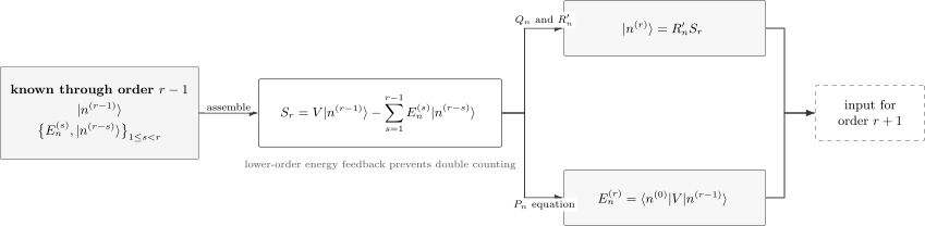
At order $r$, lower-order data form a source $S_r$. Its $P_n$ projection fixes $E_n^{(r)}$, while its $Q_n$ projection is propagated by the reduced resolvent to produce $\lvert n^{(r)}\rangle$. The energy-feedback terms remove components already generated at lower orders.

A Practical Recursion in Components

Suppose the $H_0$ eigenbasis has been truncated to a finite set for computation. Write

$$c_m^{(r)} = \langle m^{(0)}\vert n^{(r)}\rangle, \qquad c_m^{(0)}=\delta_{mn}.$$

At each order $r$:

1. Compute the energy coefficient

   $$E_n^{(r)} = \sum_m V_{nm}c_m^{(r-1)}.$$

2. Form the source components

   $$b_m^{(r)} = \sum_kV_{mk}c_k^{(r-1)} - \sum_{s=1}^{r-1} E_n^{(s)}c_m^{(r-s)}.$$

3. Resolve the complementary component:

   $$c_m^{(r)} = \frac{b_m^{(r)}} {E_n^{(0)}-E_m^{(0)}}, \qquad m\ne n,$$

   and set $c_n^{(r)}=0$.

This implementation needs matrix–vector products and stored lower-order vectors. It avoids explicitly generating the rapidly expanding closed-form sums. In a large sparse basis, applying $V$ and solving the projected linear equation can be preferable to constructing $R_n'$ as a dense matrix.

For a Hamiltonian with explicit higher powers,

$$H(\lambda) = H_0+ \sum_{j\ge1}\lambda^jV_j,$$

replace $V\lvert n^{(r-1)}\rangle$ by

$$\sum_{j=1}^{r} V_j\lvert n^{(r-j)}\rangle.$$

The energy recursion then becomes

$$E_n^{(r)} = \sum_{j=1}^{r} \langle n^{(0)}\rvert V_j \lvert n^{(r-j)}\rangle.$$

This distinction matters when the physical Hamiltonian itself has a quadratic or higher-order dependence on the expansion parameter.

Third-Order Anatomy

Define

$$\begin{aligned} \Delta_{nm} &\equiv E_n^{(0)}-E_m^{(0)}, \\ V_{mk} &\equiv \langle m^{(0)}\rvert V \lvert k^{(0)}\rangle. \end{aligned}$$

The first two energy coefficients are

$$\begin{aligned} E_n^{(1)} &=V_{nn}, \\ E_n^{(2)} &= \sum_{m\ne n} \frac{V_{nm}V_{mn}}{\Delta_{nm}}. \end{aligned}$$

One more use of the recursion gives

$$\begin{aligned} E_n^{(3)} ={}& \sum_{m\ne n} \sum_{k\ne n} \frac{ V_{nm}V_{mk}V_{kn} }{ \Delta_{nm}\Delta_{nk} } \\ &- V_{nn} \sum_{m\ne n} \frac{ V_{nm}V_{mn} }{ \Delta_{nm}^{,2} }. \end{aligned}$$

The first term is a chain of three perturbation insertions,

$$n\longrightarrow k\longrightarrow m\longrightarrow n,$$

summed over intermediate states. The second is a subtraction term. It is not an optional normalization adjustment: it is required by the feedback of the first-order energy into the second-order state equation.

If $V_{nn}=0$, the subtraction term vanishes, but the double sum generally remains. Selection rules may remove additional chains. For example, if $H_0$ is parity invariant, the reference level has definite parity, and $V$ is parity odd, then every odd-order energy correction vanishes. The strongest argument is not term-by-term cancellation: parity maps $H(\lambda)$ to $H(-\lambda)$, so an isolated eigenvalue branch satisfies $E_n(\lambda)=E_n(-\lambda)$.

At fourth order, several chain topologies and several feedback products occur. The number of algebraic terms grows because an order-$r$ coefficient contains all ordered partitions of lower orders as well as sums over intermediate states. This is why recursive or diagrammatic organization becomes valuable.

Diagram-Like Bookkeeping

A typical unreduced chain at order $r$ has the schematic form

$$\frac{ V_{nm_1}V_{m_1m_2}\cdots V_{m_{r-1}n} }{ \Delta_{nm_1}\Delta_{nm_2}\cdots \Delta_{nm_{r-1}} }.$$

It can be pictured as a path that leaves the reference state, visits virtual intermediate states, and returns. That picture records four kinds of information:

• each vertex represents an insertion of $V$;
• each intermediate segment carries an energy denominator;
• sums run over labels allowed by symmetry and statistics;
• subtraction structures remove reducible or normalization-generated pieces.

This is diagram-like bookkeeping, not yet a full Feynman-diagram formalism. In many-body perturbation theory, a second-quantized basis and Wick’s Theorem Preview turn these chains into Goldstone diagrams with precise sign, symmetry-factor, and denominator rules. Time-ordered Feynman diagrams and stationary Goldstone diagrams encode related expansions, but their objects and denominators are not interchangeable without a derivation.

Diagrams are useful because many apparently different index sums share one topology. They do not eliminate the need to define the reference state, normalization convention, intermediate-state space, or denominator prescription.

Linked-Cluster Idea Preview

Consider two noninteracting subsystems,

$$\begin{aligned} H_0 &=H_{0A}+H_{0B}, \\ V &=V_A+V_B, \end{aligned}$$

acting on a product Hilbert space. Their exact energy is additive:

$$E_{AB}(\lambda) = E_A(\lambda)+E_B(\lambda).$$

Therefore every perturbative coefficient must also be additive:

$$E_{AB}^{(r)} = E_A^{(r)}+E_B^{(r)}.$$

Naively expanding a many-body wavefunction produces products in which one perturbation acts in $A$ while another acts independently in $B$. Such unlinked products cannot survive in the energy because they would violate additivity and, in a macroscopic system, produce the wrong scaling with system size. Normalization and energy-feedback terms cancel them.

The linked-cluster theorem formalizes this cancellation in many-body perturbation theory: the energy can be organized using linked contributions. In diagrammatic language, every retained energy diagram is connected to the reference structure. This preview should not be read as a proof for arbitrary Hamiltonians or as permission to discard a term merely because a hand-drawn picture looks disconnected. The precise theorem depends on the reference state, operator decomposition, and diagram rules.

The same structural lesson appears in the recursion above. Terms involving lower $E_n^{(s)}$ subtract contributions that would otherwise be counted again through lower-order state corrections. Perturbation Theory in Many-Body Systems develops the equivalent logarithm-and-cumulant organization and its volume-scaling consequences.

Normalization and Observables

Intermediate normalization gives

$$\langle n^{(0)}\vert n^{(r)}\rangle=0$$

but generally

$$\langle n(\lambda)\vert n(\lambda)\rangle \ne1.$$

Through second order,

$$\langle n(\lambda)\vert n(\lambda)\rangle = 1+ \lambda^2 \langle n^{(1)}\vert n^{(1)}\rangle +O(\lambda^3).$$

A unit-normalized state therefore begins with the normalization factor

$$\mathcal N_2(\lambda) = 1- \frac{\lambda^2}{2} \langle n^{(1)}\vert n^{(1)}\rangle +O(\lambda^3).$$

Thus

$$\begin{aligned} \lvert \widehat n(\lambda)\rangle ={}& \mathcal N_2(\lambda) \Bigl[ \lvert n^{(0)}\rangle +\lambda\lvert n^{(1)}\rangle \\ &\qquad+ \lambda^2\lvert n^{(2)}\rangle \Bigr] +O(\lambda^3). \end{aligned}$$

For an observable $A$, the convention-independent quantity is

$$\langle A\rangle_\lambda = \frac{ \langle n(\lambda)\rvert A \lvert n(\lambda)\rangle }{ \langle n(\lambda)\vert n(\lambda)\rangle }.$$

Expanding the numerator while forgetting the denominator creates spurious higher-order terms. Energy coefficients are especially simple in intermediate normalization because the projection formula already contains the required feedback.

Convergence Is Controlled by Analytic Structure

For a finite-dimensional matrix $H(\lambda)$ whose entries are analytic in $\lambda$, a simple eigenvalue admits a local analytic branch. Its Taylor series stops converging when analytic continuation encounters the nearest singularity in the complex $\lambda$ plane. That singularity is often an exceptional point where two eigenvalues and their projectors coalesce.

Real-axis level spacings alone do not determine the convergence radius. A Hamiltonian can be Hermitian for every real $\lambda$ and still have nearby branch points at complex $\lambda$.

Worked Example: An Exactly Solvable Two-Level Model

Take

$$H(\lambda) = \begin{pmatrix} 0 & \lambda v \\ \lambda v & \Delta \end{pmatrix}, \qquad \Delta\gt0,$$

with real $v$. The lower eigenvalue is

$$E_-(\lambda) = \frac{ \Delta- \sqrt{\Delta^2+4\lambda^2v^2} }{2}.$$

Expanding about $\lambda=0$ gives

$$\begin{aligned} E_-(\lambda) ={}& -\frac{v^2}{\Delta}\lambda^2 +\frac{v^4}{\Delta^3}\lambda^4 \\ &- \frac{2v^6}{\Delta^5}\lambda^6 + \frac{5v^8}{\Delta^7}\lambda^8 +\cdots. \end{aligned}$$

The square root has branch points at

$$\lambda_\star = \pm i\frac{\Delta}{2v}.$$

Hence the Taylor series converges only for

$$\lvert\lambda\rvert \lt \frac{\Delta}{2\lvert v\rvert}.$$

The exact eigenvalue remains perfectly finite for all real $\lambda$. The obstruction is a complex degeneracy, not a real-axis divergence. Exact diagonalization of this two-state subspace automatically continues beyond the perturbative disk and is the correct cure when $\lvert\lambda v\rvert$ is no longer small compared with $\Delta$.

Asymptotic Series

An expansion can accurately describe a function near $\lambda=0$ without converging for any nonzero $\lambda$. The notation

$$E(\lambda) \sim \sum_{r=0}^{\infty}a_r\lambda^r$$

means that, for every fixed $N$ in the relevant sector,

$$E(\lambda) - \sum_{r=0}^{N}a_r\lambda^r = o(\lambda^N)$$

as $\lambda\to0$. It does not assert convergence as $N\to\infty$ at fixed nonzero $\lambda$.

Many quantum-mechanical perturbation series have coefficients with factorial large-order growth, schematically

$$a_r \sim C A^{-r}\Gamma(r+b).$$

Then the terms initially decrease but eventually grow. Their ratio behaves roughly as

$$\left| \frac{a_{r+1}\lambda^{r+1}} {a_r\lambda^r} \right| \sim \frac{\lvert\lambda\rvert}{\lvert A\rvert} (r+b).$$

The smallest term occurs near

$$r_{\mathrm{opt}} \sim \frac{\lvert A\rvert}{\lvert\lambda\rvert}.$$

Truncating near that least term often gives the best raw partial sum. Adding terms beyond it makes the approximation worse even though each coefficient has been computed correctly.

The quartic anharmonic oscillator,

$$\begin{aligned} H(g) &= \frac{p^2}{2m} + \frac12m\omega^2x^2 +gx^4, \\ g&\gt0, \end{aligned}$$

is the canonical example. Its ordinary weak-coupling energy series is divergent but asymptotic; in the standard stable problem it is recoverable by appropriate summation methods. The large-order behavior is tied to the analytic continuation toward negative coupling, where the potential is unstable. Anharmonic Oscillator develops the model, Asymptotic Series and Nonperturbative Corrections derives optimal truncation and the least-term scale, Variational Perturbation Theory develops an order-dependent reorganization, and Resurgence Preview introduces Borel and nonperturbative structure cautiously.

Three lessons are worth keeping separate:

• divergent does not mean numerically useless;
• convergent does not mean rapidly convergent at the desired coupling;
• high-order coefficients can contain information about singularities and nonperturbative scales, but extracting that information requires more than forming a long partial sum.

When Higher Order Is Useful

Computing another order is well motivated when:

• a dimensionless mixing parameter is clearly small and the observed term sequence decreases;
• symmetry or a selection rule forces the lower-order coefficients to vanish;
• the desired precision is finer than the first omitted term;
• an analytic coefficient is itself the observable of interest, as in a susceptibility or response derivative;
• parameter dependence and physical interpretation matter more than a single numerical value;
• a high-accuracy numerical result is available and perturbation theory is being used as an independent benchmark;
• large-order behavior is the subject of study rather than merely a route to a low-order estimate.

Higher order is most valuable when accompanied by a control diagnostic. Merely having an algebra system capable of producing more terms is not such a diagnostic.

When Diagonalization Is Better

The question is not whether perturbation theory or diagonalization is universally superior. They answer different needs.

• One or a few nearby levels dominate: diagonalize that subspace. This treats avoided crossings and repeated mixing nonperturbatively.
• Many ratios $\lvert\lambda V_{mn}/\Delta_{nm}\rvert$ are not small: enlarge the exact model space. No reliable hierarchy separates successive orders.
• A modest converged basis matrix is available: use numerical eigensolvers. A full eigenpair may cost less than high-order symbolic sums.
• Lower orders vanish by symmetry and the next order is sparse: continue perturbatively. The analytic coefficient remains compact and informative.
• The series is asymptotic but terms are still decreasing: truncate near the least term. Early orders can be highly accurate.
• Terms have begun growing: stop the raw series. More coefficients do not improve the partial sum.
• Continuum thresholds or resonances are nearby: reformulate the spectral problem. A bound-state power series may describe the wrong analytic object.

Matrix Diagonalization covers finite Hermitian eigensolvers and residual checks. Near degeneracy, Degenerate Perturbation Theory or a projected effective Hamiltonian is usually preferable to pushing a one-state expansion to high order. Brillouin–Wigner Perturbation Theory keeps the unknown energy in the resolvent and thereby resums selected denominator effects.

Even when diagonalization supplies the final number, low-order perturbation theory remains useful for identifying dominant couplings, symmetry constraints, parameter scaling, and basis-convergence errors.

Validation and Stopping Rules

Let the order-$N$ approximants be

$$\begin{aligned} E_n^{[N]}(\lambda) &= \sum_{r=0}^{N} \lambda^rE_n^{(r)}, \\ \lvert n^{[N]}(\lambda)\rangle &= \sum_{r=0}^{N} \lambda^r \lvert n^{(r)}\rangle. \end{aligned}$$

Useful checks include:

1. Term size. Inspect

   $$T_r(\lambda)=\lambda^rE_n^{(r)}.$$

   A decreasing sequence supports continued truncation locally; a growing sequence is a warning, not proof by itself, that the useful asymptotic window has passed.

2. Successive approximants. Compare $E_n^{[N]}$ and $E_n^{[N-1]}$. Their difference is the last included term, not a rigorous error bar unless additional remainder information is available.

3. Eigenpair residual. Compute

   $$\mathcal R_N = \bigl(H(\lambda)-E_n^{[N]}(\lambda)\bigr) \lvert n^{[N]}(\lambda)\rangle.$$

   Exact coefficient matching makes this formally $O(\lambda^{N+1})$, but a numerical residual also contains basis truncation and roundoff errors.

4. Basis stability. Increase the intermediate-state cutoff independently of perturbative order. Agreement in $N$ with a fixed inadequate basis is not convergence to the continuum problem.

5. Symmetry checks. Forbidden coefficients should vanish to numerical precision. A small nonzero value can expose a basis, quadrature, or implementation error.

6. Exact subspace comparison. Diagonalize the smallest subspace containing the strongly mixed states and compare its Taylor coefficients with the recursion.

7. Independent benchmark. Compare with a variational bound, direct shooting calculation, spectral discretization, or trusted exact result where available. The Perturbation-Theory Benchmarks Notebook is the natural home for reproducible comparisons.

A practical stopping rule for an asymptotic sequence is to stop at or just before the smallest observed term, provided basis and roundoff errors are smaller. For a genuinely convergent series, ratio estimates from several late coefficients can suggest the convergence radius, but a short coefficient list rarely establishes it reliably.

Boundaries of the Recursion

The formulas on this page require modification when:

• the target eigenvalue is degenerate or nearly degenerate;
• the eigenvalue is embedded in a continuum or becomes a resonance;
• $V$ changes the operator domain in a singular way;
• the desired branch is not analytic in the chosen parameter;
• the reference overlap vanishes, so intermediate normalization breaks down;
• the state is tracked through a level collision without a branch convention;
• ultraviolet sums diverge and require a regulator, renormalization, or a better effective description.

An isolated eigenvalue and a small real coupling are not by themselves a proof of convergence. Rigorous analytic perturbation theory requires hypotheses about the operator family, domains, spectral isolation, and relative boundedness or quadratic-form control. Kato’s operator theory is the standard mathematical reference.

Common Mistakes

• Memorizing a fourth-order formula without stating the normalization convention.
• Treating every repeated matrix-element chain as an independent contribution and omitting feedback subtractions.
• Assuming Hermiticity on the real axis guarantees an infinite convergence radius.
• Equating a divergent series with a failed approximation.
• Adding terms after an asymptotic series has passed its least term.
• Using a one-state recursion across a near-degeneracy.
• Confusing perturbative-order convergence with basis-set convergence.
• Calling a sketch a linked-cluster proof without defining the diagram rules.
• Expanding an observable numerator while forgetting the state norm.
• Reporting the last retained term as a rigorous uncertainty without a remainder theorem.

Exercises

1. Derive the two recursions

Starting from the coefficient equation at order $r$, derive the energy and state recursions under intermediate normalization.

Solution

The order-$r$ equation is

$$\begin{aligned} \bigl(H_0-E_n^{(0)}\bigr) \lvert n^{(r)}\rangle ={}& -V\lvert n^{(r-1)}\rangle \\ &+ \sum_{s=1}^{r} E_n^{(s)} \lvert n^{(r-s)}\rangle. \end{aligned}$$

Left multiplication by $\langle n^{(0)}\rvert$ kills the left side. Intermediate normalization kills every term in the sum except $s=r$, for which $\lvert n^{(r-s)}\rangle=\lvert n^{(0)}\rangle$. Thus

$$E_n^{(r)} = \langle n^{(0)}\rvert V \lvert n^{(r-1)}\rangle.$$

Multiplying the original equation by $-1$, projecting with $Q_n$, and applying $Q_n(E_n^{(0)}-H_0)^{-1}Q_n$ gives

$$\begin{aligned} \lvert n^{(r)}\rangle =R_n'\Biggl[ &V\lvert n^{(r-1)}\rangle \\ &- \sum_{s=1}^{r-1} E_n^{(s)} \lvert n^{(r-s)}\rangle \Biggr]. \end{aligned}$$

The $s=r$ term is proportional to $\lvert n^{(0)}\rangle$ and is annihilated by $R_n'P_n=0$.

2. Recover the third-order energy

Use the recursion to derive the displayed expression for $E_n^{(3)}$.

Solution

The first-order state is

$$\lvert n^{(1)}\rangle = \sum_{k\ne n} \frac{V_{kn}}{\Delta_{nk}} \lvert k^{(0)}\rangle.$$

At second order,

$$\lvert n^{(2)}\rangle = R_n' \bigl(V-E_n^{(1)}\bigr) \lvert n^{(1)}\rangle.$$

Therefore, for $m\ne n$,

$$\langle m^{(0)}\vert n^{(2)}\rangle = \sum_{k\ne n} \frac{V_{mk}V_{kn}} {\Delta_{nm}\Delta_{nk}} - \frac{V_{nn}V_{mn}} {\Delta_{nm}^{,2}}.$$

Finally,

$$E_n^{(3)} = \langle n^{(0)}\rvert V \lvert n^{(2)}\rangle,$$

which yields

$$\begin{aligned} E_n^{(3)} ={}& \sum_{m,k\ne n} \frac{V_{nm}V_{mk}V_{kn}} {\Delta_{nm}\Delta_{nk}} \\ &- V_{nn} \sum_{m\ne n} \frac{V_{nm}V_{mn}} {\Delta_{nm}^{,2}}. \end{aligned}$$

3. Odd perturbation and odd orders

Let $\Pi H_0\Pi^{-1}=H_0$ and $\Pi V\Pi^{-1}=-V$, where $\Pi$ is parity. Show that all odd energy coefficients vanish for an isolated branch.

Solution

Parity transforms the full Hamiltonian as

$$\Pi H(\lambda)\Pi^{-1} = H(-\lambda).$$

Unitary equivalence preserves the spectrum. For an isolated branch that is continuously identified with the same unperturbed eigenvalue,

$$E_n(\lambda)=E_n(-\lambda).$$

Its Taylor expansion is therefore even:

$$E_n(\lambda) = E_n^{(0)} +\lambda^2E_n^{(2)} +\lambda^4E_n^{(4)} +\cdots.$$

Hence $E_n^{(2j+1)}=0$ for every $j\ge0$. This symmetry argument is stronger and cleaner than checking individual chains.

4. Two-level convergence radius

For the two-level model in the worked example, find the branch points and verify the first four nonzero perturbative terms.

Solution

The discriminant vanishes when

$$\Delta^2+4\lambda^2v^2=0,$$

so

$$\lambda_\star = \pm i\frac{\Delta}{2v}.$$

The nearest singularities are a distance $\Delta/(2\lvert v\rvert)$ from the origin. Write

$$E_-(\lambda) = \frac{\Delta}{2} \left[ 1- \sqrt{1+ \frac{4\lambda^2v^2}{\Delta^2}} \right].$$

Using

$$\begin{aligned} \sqrt{1+x} ={}& 1+ \frac{x}{2} - \frac{x^2}{8} \\ &+ \frac{x^3}{16} - \frac{5x^4}{128} +\cdots \end{aligned}$$

gives

$$\begin{aligned} E_-(\lambda) ={}& -\frac{v^2}{\Delta}\lambda^2 +\frac{v^4}{\Delta^3}\lambda^4 \\ &- \frac{2v^6}{\Delta^5}\lambda^6 + \frac{5v^8}{\Delta^7}\lambda^8 +\cdots. \end{aligned}$$

5. Normalize the state through second order

Given an intermediate-normalized state through $O(\lambda^2)$, derive the parallel normalization correction in the unit-normalized state.

Solution

Intermediate normalization gives

$$\langle n^{(0)}\vert n^{(1)}\rangle = \langle n^{(0)}\vert n^{(2)}\rangle =0.$$

Therefore

$$\lVert n(\lambda)\rVert^2 = 1+ \lambda^2 \langle n^{(1)}\vert n^{(1)}\rangle +O(\lambda^3).$$

Since $(1+x)^{-1/2}=1-x/2+O(x^2)$,

$$\frac{1}{\lVert n(\lambda)\rVert} = 1- \frac{\lambda^2}{2} \langle n^{(1)}\vert n^{(1)}\rangle +O(\lambda^3).$$

Multiplication by the intermediate-normalized series adds the parallel term

$$-\frac{\lambda^2}{2} \langle n^{(1)}\vert n^{(1)}\rangle \lvert n^{(0)}\rangle$$

to the state at second order.

6. Additivity and unlinked terms

For two noninteracting subsystems with $H(\lambda)=H_A(\lambda)+H_B(\lambda)$, explain why an energy term proportional to $E_A^{(1)}E_B^{(1)}$ cannot remain in $E_{AB}^{(2)}$.

Solution

The exact product eigenstate has energy

$$E_{AB}(\lambda) = E_A(\lambda)+E_B(\lambda).$$

Matching powers of $\lambda$ gives

$$E_{AB}^{(2)} = E_A^{(2)}+E_B^{(2)}.$$

A product $E_A^{(1)}E_B^{(1)}$ is not additive and would scale incorrectly when independent copies of the system are combined. Such products can appear in intermediate wavefunction or norm expansions, but energy-feedback and normalization terms cancel them. This elementary factorization check is the physical core of linked-cluster cancellations.

Cross-Links

• Nondegenerate Perturbation Theory for the basic isolated-level framework.
• Second-Order Energy Corrections for virtual mixing, signs, polarizability, and sum-over-states convergence.
• Degenerate Perturbation Theory for exact treatment inside a degenerate model space.
• Quasi-Degenerate Perturbation Theory for nearby clusters and avoided crossings.
• Brillouin–Wigner Perturbation Theory for an energy-dependent resolvent and partial resummation.
• Rayleigh–Schrödinger Perturbation Theory for the named energy-independent formalism, normalization convention, and applications.
• Small Parameters and Error Estimates for control parameters and remainder discipline.
• Anharmonic Oscillator for the standard large-order laboratory.
• Asymptotic Series and Nonperturbative Corrections for factorial growth, optimal truncation, and beyond-all-orders effects.
• Resurgence Preview for Borel transforms and perturbative–nonperturbative relations.
• Matrix Diagonalization for finite-basis eigenvalue computation and residual checks.

References

• T. Kato, Perturbation Theory for Linear Operators, 2nd ed., Springer, 1976; reprint 1995, doi:10.1007/978-3-642-66282-9.
• A. Messiah, Quantum Mechanics, Vol. II, North-Holland, 1962, Chapter XVII.
• C. Cohen-Tannoudji, B. Diu, and F. Laloë, Quantum Mechanics, Vol. II, Wiley, 1977, Complement B.
• J. J. Sakurai and J. Napolitano, Modern Quantum Mechanics, 3rd ed., Cambridge University Press, 2021, Chapter 5.
• C. M. Bender and T. T. Wu, “Anharmonic Oscillator,” Physical Review 184, 1231–1260 (1969), doi:10.1103/PhysRev.184.1231.
• C. M. Bender and T. T. Wu, “Anharmonic Oscillator. II. A Study of Perturbation Theory in Large Order,” Physical Review D 7, 1620–1636 (1973), doi:10.1103/PhysRevD.7.1620.
• B. Simon, “Coupling Constant Analyticity for the Anharmonic Oscillator,” Annals of Physics 58, 76–136 (1970), doi:10.1016/0003-4916(70)90240-X.
• J. Goldstone, “Derivation of the Brueckner Many-Body Theory,” Proceedings of the Royal Society A 239, 267–279 (1957), doi:10.1098/rspa.1957.0037.
• I. Shavitt and R. J. Bartlett, Many-Body Methods in Chemistry and Physics, Cambridge University Press, 2009, Chapters 3–5.