Spectroscopy

Spectroscopy studies a physical system through radiation that it absorbs, emits, scatters, or otherwise modifies. A spectrum is not a photograph of an energy-level diagram. It is a measured response, plotted against frequency, angular frequency, vacuum wavenumber, wavelength, photon energy, magnetic field, or another controlled variable, after state preparation, interaction, propagation, detection, and data processing.

The central inference has several layers:

$$\begin{gathered} \text{state structure} \\ \downarrow \\ \text{allowed transitions} \\ \downarrow \\ \text{response of the sample} \\ \downarrow \\ \text{recorded signal}. \end{gathered}$$

Each arrow carries assumptions. Energy differences locate ideal resonances. Matrix elements and populations control strengths. Dynamics and environments produce widths and shifts. The instrument filters the result. A trustworthy spectroscopic claim states which layer has actually been inferred.

Enter This Chapter

Use this overview first to identify what a measured spectrum can and cannot establish. Then follow the shortest route that matches the quantity you need.

Predict a rate or an integrated intensity. Start with Transition Rates, then choose Oscillator Strengths or Einstein Coefficients for the relevant convention. Absorption and Emission connects those quantities to measured signals.

Decide whether a line appears and what its width means. Use Selection Rules in Spectroscopy for symmetry permissions and Line Shapes and Broadening for lifetime, dephasing, collision, Doppler, and instrumental contributions.

Assign molecular structure. Follow Rotational Spectroscopy or Vibrational Spectroscopy, then use Infrared or Raman Spectroscopy according to the interaction operator and selection rules. For electronic and vibronic structure, continue to Electronic Spectroscopy and Fluorescence and Phosphorescence.

Probe ionization or spin dynamics. Choose Photoelectron Spectroscopy for ionized final states and Magnetic Resonance for spin precession, relaxation, and resonance conventions.

Resolve dynamics or pursue extreme accuracy. Ultrafast Spectroscopy organizes pump–probe and coherent time-domain measurements. Precision Spectroscopy organizes clocks, systematic shifts, uncertainty budgets, and tests of fundamental physics.

Check terminology or experimental practice. Use Spectroscopy Nomenclature for the compact convention ledger and Spectroscopy as an Experimental Technique for instruments, calibration, resolution, and the historical evidence chain.

You are ready to leave this overview when you can name the prepared state and populations, interaction operator and polarization, measured observable and scan coordinate, sources of position and line-shape information, instrument response, leading uncertainty, and the specialist page that owns the next calculation.

Canonical Scope

This page owns the chapter-level dictionary connecting:

• line positions to energy differences and shifts;
• amplitudes to interaction operators and symmetry;
• integrated strengths to matrix elements, populations, and conventions;
• lifetimes and dephasing to linewidths under stated dynamical assumptions;
• atomic and molecular structure to characteristic spectral organization;
• time-domain signals to frequency-domain response through Fourier analysis.

Detailed derivations and experimental histories remain in their canonical homes:

• Spectroscopy as an Experimental Technique owns dispersive instruments, resolution, calibration, and the historical evidence pipeline.
• First-Order Transition Probability owns the perturbative amplitude derivation.
• Fermi’s Golden Rule owns the long-time continuum rate limit.
• Transition Rates in Light–Matter Interaction owns the bridge from dipole coupling to absorption, stimulated emission, and spontaneous emission.
• Selection Rules and Molecular Symmetry own the general and molecular symmetry tests.
• Fourier Transform owns transform conventions and the underlying mathematics.
• Open Quantum Systems owns reduced dynamics, decoherence, and master-equation structure.

Later pages in this chapter specialize the dictionary to transition rates, oscillator strengths, Einstein coefficients, absorption and emission, line shapes, selection rules, rotational spectroscopy, vibrational spectra, Raman spectroscopy, electronic spectroscopy, fluorescence and phosphorescence, and photoelectron spectra, magnetic resonance, ultrafast measurements, and precision spectroscopy.

The Measurement Chain

A measured spectrum depends on more than the isolated-system Hamiltonian. A minimal forward model has five parts.

State preparation

Specify the initial density operator, ensemble, temperature, polarization, spatial distribution, and any coherences. For a thermal ensemble,

$$p_i = \frac{ g_i e^{-E_i/(k_{\mathrm B}T)} }{ \displaystyle \sum_j g_j e^{-E_j/(k_{\mathrm B}T)} },$$

where $g_i$ is the degeneracy included in the chosen level definition. Here $p_i$ is the total population of level $i$, not the population of one degenerate substate. The formula assumes equal thermal population within that level. Nonthermal optical pumping, state selection, chemical kinetics, and population inversion require a different preparation model and may require substate-resolved populations.

Interaction

Identify the operator that couples the probe to the system. Examples include:

• an electric dipole for leading optical absorption;
• a magnetic dipole for magnetic resonance;
• a polarizability tensor for nonresonant Raman scattering;
• a photoionization operator for electron spectroscopy;
• a density or spin operator for scattering probes.

The word “spectrum” does not determine the operator.

Evolution

During and after the interaction, the system may undergo coherent motion, spontaneous decay, collisions, dephasing, transport, or chemical conversion. These processes can alter the measured line before the detector receives a signal.

Detection

The detector may count photons or particles, measure transmitted power, heterodyne a field quadrature, record fluorescence versus time, or infer a population after a pulse sequence. Distinct detection observables can assign different weights to the same underlying transitions.

Instrument response and inference

Calibration, sampling, finite resolution, background subtraction, and the chosen fit model map the physical response to reported parameters. A compact description is

$$\begin{aligned} S_{\mathrm{obs}}(x) &= \int R(x,x') \\ &\qquad {}\times S_{\mathrm{sample}}(x')\, dx' + B(x), \end{aligned}$$

where $x$ is the plotted coordinate, $R$ is the instrument response, and $B$ is a background model. Deconvolution is an inverse problem, not a purely graphical sharpening operation.

Spectra as Energy Differences

Transition frequencies

Let the unperturbed system satisfy

$$\widehat H_0|n\rangle = E_n|n\rangle.$$

For a transition from $|i\rangle$ to $|f\rangle$, define the signed Bohr angular frequency

$$\omega_{fi} = \frac{E_f-E_i}{\hbar}.$$

Absorption from a lower to a higher state requires positive photon energy:

$$E_f-E_i = \hbar\omega >0.$$

Emission from an upper state $|u\rangle$ to a lower state $|\ell\rangle$ produces

$$\hbar\omega = E_u-E_\ell >0.$$

The measured positive photon frequency should not be confused with a signed index convention such as $\omega_{fi}$.

Frequency, wavenumber, wavelength, and energy

For propagation in vacuum,

$$\Delta E = h\nu = \hbar\omega = hc_0\widetilde\nu,$$

with

$$\omega=2\pi\nu, \qquad \widetilde\nu = \frac{\nu}{c_0} = \frac{1}{\lambda_0}.$$

Here $\widetilde\nu$ is vacuum wavenumber and $\lambda_0$ is vacuum wavelength. The common spectroscopic unit $\mathrm{cm}^{-1}$ is a wavenumber, not a frequency. In a material medium, wavelength depends on refractive index, so conventions must be stated.

Peak coordinates transform straightforwardly, but spectral densities do not. If $S_\nu(\nu)\,d\nu$ and $S_\lambda(\lambda)\,|d\lambda|$ describe the same integrated signal, then

$$S_\lambda(\lambda) = S_\nu\!\left(\frac{c_0}{\lambda}\right) \frac{c_0}{\lambda^2}.$$

A symmetric line in frequency is therefore not exactly symmetric in wavelength. Comparing peak heights or integrated areas across axes requires the Jacobian.

A spectrum contains transitions, not levels

With $N$ levels there can be as many as $N(N-1)/2$ positive pairwise energy differences before selection rules and preparation are imposed. Conversely, several transitions can coincide at one frequency.

For three ordered levels $E_0<E_1<E_2$,

$$\nu_{20} = \nu_{21} + \nu_{10}.$$

Such combination differences help construct a self-consistent level scheme. They also show why one peak does not by itself identify two absolute energies. A common additive shift of all $E_n$ leaves every transition frequency unchanged.

Discrete lines and continua

Bound-to-bound transitions produce discrete ideal frequencies. Bound-to-free photoionization and scattering channels have continuum final energies. Dense rovibronic structure, disorder, short lifetimes, and unresolved components can make a discrete manifold look band-like.

A continuous measured spectrum does not prove that the underlying Hamiltonian has no discrete states, and a sharp line does not prove that the system is perfectly isolated.

The line center is model dependent

The simple relation $\hbar\omega_{fi}=E_f-E_i$ uses a specified Hamiltonian. Observed centers can include:

• fine, hyperfine, and isotope shifts;
• Zeeman and Stark shifts;
• recoil and relativistic Doppler effects;
• pressure and collisional shifts;
• radiative corrections;
• mean-field or many-body shifts;
• calibration offsets and unresolved blends.

A precision line center is therefore a comparison between a forward model and data, not an unqualified reading of “the energy difference.”

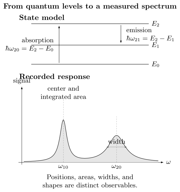
From a level model to a measured response. Transition energies set ideal centers; the interaction operator and preparation determine which arrows carry weight; dynamics, environment, and apparatus determine each peak’s width and shape.

Transition Amplitudes and Selection Rules

First-order amplitude

Write

$$\widehat H(t) = \widehat H_0 + \widehat V(t).$$

If the system begins in $|i\rangle$, first-order time-dependent perturbation theory gives

$$c_f^{(1)}(t) = -\frac{i}{\hbar} \int_{t_0}^{t} dt'\, e^{i\omega_{fi}t'} \langle f| \widehat V(t') |i\rangle.$$

This formula separates three ingredients:

• the state’s Bohr phase $e^{i\omega_{fi}t'}$;
• the interaction matrix element;
• the temporal spectrum of the applied field.

For a finite pulse, the transition probability has finite bandwidth. Exact energy-conserving delta functions arise only after an appropriate long-time or continuum limit.

Electric-dipole example

In the long-wavelength electric-dipole approximation,

$$\widehat V(t) = -\widehat{\mathbf d} \cdot \mathbf E(t).$$

For polarization unit vector $\boldsymbol\epsilon$, the relevant material amplitude contains

$$\boldsymbol\epsilon \cdot \mathbf d_{fi}, \qquad \mathbf d_{fi} = \langle f| \widehat{\mathbf d} |i\rangle.$$

Changing polarization can suppress one magnetic sublevel channel and enhance another without changing the field-free level energies.

Selection rules are matrix-element statements

A selection rule says that a matrix element vanishes under stated symmetry and model assumptions. In representation language,

$$\Gamma_f^* \otimes \Gamma_O \otimes \Gamma_i \supset \Gamma_{\mathrm{triv}}$$

is necessary for a nonzero matrix element of operator $\widehat O$, where $\Gamma_{\mathrm{triv}}$ is the totally symmetric, or trivial, representation. It is a permission test, not a sufficiency theorem: dynamics, additional symmetries, or accidental cancellation can still make an allowed matrix element vanish.

This statement must name:

• the symmetry group;
• the initial and final state labels;
• the transition operator and multipole order;
• any angular-momentum coupling approximation;
• external fields or symmetry-breaking environments.

“Allowed” means not forced to zero. It does not mean intense. “Forbidden” means zero in the stated approximation, not impossible under every interaction.

From amplitudes to rates

For weak coupling to a continuum of final states, the golden-rule structure is

$$\Gamma_{i\rightarrow f} = \frac{2\pi}{\hbar} \left| V_{fi} \right|^2 \rho(E_f),$$

with normalization, degeneracy sums, field factors, and the density of states defined consistently. The rule is not a universal formula for every spectral peak. Short pulses, strong driving, discrete final states, coherent interference, and non-Markovian dynamics require their own treatments.

Response functions

In linear response, a weak generalized force $F(t)$ coupled to an operator $\widehat B$ induces

$$\delta\langle A(t)\rangle = \int_{-\infty}^{\infty} dt'\, \chi_{AB}(t-t')F(t').$$

Causality gives $\chi_{AB}(t<0)=0$. In frequency space,

$$\delta A(\omega) = \chi_{AB}(\omega)F(\omega).$$

The absorptive part of a susceptibility, a transition-rate sum, and a correlation spectrum are related descriptions in their shared regime, but their normalization and sign conventions are not interchangeable without a derivation.

Intensities and Lifetimes

A strength dictionary

Several quantities called “intensity” encode different objects:

• peak height depends strongly on linewidth and resolution;
• integrated line area removes profile normalization but still depends on the plotted variable;
• line strength is commonly a squared transition matrix element with a stated angular convention;
• oscillator strength is dimensionless and includes energy and degeneracy factors;
• Einstein $A$ coefficient is a spontaneous-emission rate;
• Einstein $B$ coefficients multiply a specified radiation energy density;
• cross section converts incident flux into a rate;
• absorbance, absorptance, and transmittance are distinct measured quantities.

Never compare two published “intensities” until their definitions, units, degeneracy averages, polarization sums, and integration variables agree.

A schematic weak spectrum

For isolated, noninterfering lines, a useful orientation model is

$$S(\omega) = \sum_{i,f} p_i\, \mathcal S_{if}\, L_{if} \left( \omega-\omega_{fi} \right),$$

where:

• $p_i$ is the prepared total population of initial level $i$;
• $\mathcal S_{if}$ contains the operator and polarization factors and uses a declared degeneracy convention;
• $L_{if}$ is a normalized line profile;
• $\omega_{fi}$ is the center in the chosen model.

For the level-population convention above, equal population of unresolved initial substates and unresolved detection of final substates give, schematically,

$$\mathcal S_{if} = \frac{1}{g_i} \sum_{\alpha=1}^{g_i} \sum_{\beta=1}^{g_f} \left| \langle f,\beta|\widehat O|i,\alpha\rangle \right|^2.$$

The factor $g_i$ must not be inserted again after it has already entered the total thermal population $p_i$. Polarized or substate-selected preparation requires the resolved populations and matrix elements instead of this average.

This is not universal. Coherent pathways add amplitudes before squaring. Overlapping resonances can interfere. Saturation makes populations depend on the drive. Many-body spectra can contain continua without a one-line decomposition.

Populations and detailed balance

In thermal equilibrium,

$$\frac{p_f}{p_i} = \frac{g_f}{g_i} \exp \left[ -\frac{E_f-E_i} {k_{\mathrm B}T} \right].$$

Absorption strength therefore changes with temperature even when the Hamiltonian and transition matrix elements do not. Hot bands, stimulated emission, nuclear-spin statistical weights, and partition functions all enter quantitative molecular spectra.

In an optically thin emission measurement, a line’s radiated power is proportional to the upper-state population, photon energy, and spontaneous rate:

$$P_{u\ell} \propto N_u\, \hbar\omega_{u\ell}\, A_{u\ell}.$$

This is why a strong emission line need not have the largest transition probability: the emitting population can dominate.

Lifetimes and branching fractions

If an excited state $u$ decays through independent weak channels,

$$\Gamma_u = \sum_{\ell} A_{u\ell} + \Gamma_u^{\mathrm{nr}}, \qquad \tau_u = \frac{1}{\Gamma_u}.$$

The branching fraction for radiative channel $u\to\ell$ is

$$b_{u\ell} = \frac{A_{u\ell}}{\Gamma_u}.$$

The radiative quantum yield is

$$\Phi_{\mathrm{rad}} = \frac{ \displaystyle\sum_\ell A_{u\ell} }{ \Gamma_u }.$$

These formulas assume an exponential population decay with time-independent rates. State mixing, trapping, reabsorption, time-dependent environments, and nonexponential kinetics require a broader model.

Weak and strong probing

In the weak-probe regime, the signal is linear in probe intensity and the initial populations are approximately unchanged. Stronger driving can cause:

• depletion or optical pumping;
• stimulated emission;
• saturation and power broadening;
• Rabi oscillations;
• AC Stark shifts;
• multiphoton transitions;
• coherent population trapping.

A line strength inferred from saturated data requires a dynamical fit, not a linear extrapolation by assumption.

Line Shapes

Center, area, width, and shape

Write one isolated contribution as

$$\begin{aligned} S(\omega) &= \mathcal A\, L(\omega-\omega_0), \\ \int_{-\infty}^{\infty} L(\delta\omega)\, d\delta\omega &= 1. \end{aligned}$$

Then $\mathcal A$ is the integrated area on the angular-frequency axis. The profile $L$ determines peak height, width, wings, and symmetry. Reporting only a fitted center discards dynamical information; reporting only a width without its convention is ambiguous.

Lorentzian profile

A normalized Lorentzian with half width at half maximum $\gamma$ is

$$L_{\mathrm L}(\delta\omega) = \frac{1}{\pi} \frac{\gamma} {\delta\omega^2+\gamma^2}.$$

Its angular-frequency full width at half maximum is

$$\Delta\omega_{\mathrm{FWHM}} = 2\gamma.$$

At fixed area, increasing $\gamma$ lowers the peak height. A broader peak is not automatically a stronger transition.

Gaussian profile

A normalized Gaussian with angular-frequency standard deviation $\sigma$ is

$$L_{\mathrm G}(\delta\omega) = \frac{1} {\sigma\sqrt{2\pi}} \exp \left( -\frac{\delta\omega^2} {2\sigma^2} \right).$$

Its full width at half maximum is

$$\Delta\omega_{\mathrm{FWHM}} = 2\sqrt{2\ln2}\,\sigma.$$

Doppler broadening from a one-dimensional Maxwell velocity distribution is Gaussian in frequency to leading nonrelativistic order, with

$$\sigma_\omega = \frac{\omega_0}{c_0} \sqrt{ \frac{k_{\mathrm B}T}{m} }.$$

Voigt and more general profiles

The convolution of a Lorentzian and a Gaussian is a Voigt profile:

$$L_{\mathrm V} = L_{\mathrm L} * L_{\mathrm G}.$$

Voigt fitting is common, but not every line is Voigt. Speed-dependent collisions, Dicke narrowing, unresolved hyperfine components, asymmetric interference, spectral diffusion, and many-body thresholds can demand more specific models.

Lifetime and coherence conventions

If the optical coherence decays as

$$\rho_{fi}(t) \propto e^{-t/T_2} e^{-i\omega_0t},$$

then its Lorentzian angular-frequency half width is $1/T_2$. For a two-level Markovian model,

$$\frac{1}{T_2} = \frac{1}{2T_1} + \frac{1}{T_\phi},$$

where $T_1$ is the population-relaxation time and $T_\phi$ is the pure dephasing time. If the lower state is stable and pure dephasing is absent,

$$\Delta\omega_{\mathrm{FWHM}} = \frac{1}{T_1}, \qquad \Delta\nu_{\mathrm{FWHM}} = \frac{1}{2\pi T_1}.$$

These are model-dependent relations, not a derivation from a vague energy–time uncertainty slogan.

Line Shapes and Broadening develops the lifetime, Doppler, collisional, power, instrumental, and beyond-Voigt models and the corresponding fitting cautions.

Broadening and shifting mechanisms

Separate at least:

• natural or radiative broadening;
• collisional broadening and pressure shifts;
• Doppler broadening;
• transit-time and finite-observation effects;
• power broadening;
• inhomogeneous static distributions;
• spectral diffusion;
• unresolved isotope, hyperfine, rotational, or site structure;
• instrumental resolution and frequency noise.

Several mechanisms can coexist. Widths add only in special parameterizations; profiles generally combine by convolution, averaging, or a joint dynamical model.

Fitting cautions

A credible line-shape analysis reports:

• the fitted coordinate and units;
• HWHM, FWHM, standard deviation, or another explicit width;
• baseline and instrument-response models;
• the fit window and treatment of neighboring lines;
• parameter covariance and residuals;
• calibration and resolution uncertainties;
• whether the profile was physically derived or chosen empirically.

A small statistical fit error does not cover model misspecification.

Atomic, Molecular, and Optical Spectra

Atomic spectra

Atomic spectra are organized by electronic configurations, term symbols, angular momentum, parity, and coupling schemes. Successive structure can include:

• gross electronic energies;
• fine structure;
• hyperfine structure;
• isotope shifts;
• Zeeman and Stark splittings;
• radiative and recoil corrections.

Atomic Physics develops the hierarchy, while Atomic Selection Rules connects it to leading transition operators. Critically evaluated wavelengths, levels, and transition probabilities should be taken from a database that states uncertainties and provenance, not from an unlabeled line list.

Rotational spectra

For an ideal linear rigid rotor,

$$E_J = BJ(J+1), \qquad J=0,1,2,\ldots,$$

with the unit convention for $B$ stated. Rotational line spacings reveal moments of inertia and isotope effects. Real spectra also contain centrifugal distortion, spin statistics, hyperfine structure, external-field shifts, and rovibrational coupling.

Rotational Spectroscopy develops the measurement, assignment, isotope-comparison, catalog, and structure-inference workflow. Rotations of Molecules owns the molecular rotor hierarchy and effective theory.

Vibrational spectra

Near a stable equilibrium, a normal mode begins with

$$E_v \approx \hbar\Omega \left( v+\frac12 \right).$$

Anharmonicity shifts level spacings and permits overtones and combination bands. Infrared activity probes dipole derivatives; nonresonant Raman activity probes polarizability derivatives. Symmetry, temperature, isotope substitution, and rovibrational coupling shape the observed band.

Normal Modes of Polyatomics owns the Hessian, mode classification, and first-order IR/Raman activity. Vibrational Spectroscopy develops the band-assignment language, anharmonic corrections, overtone and combination structure, and force-constant inference workflow. Infrared Spectroscopy develops electric-dipole coupling, FTIR and ATR measurement models, rovibrational envelopes, and fingerprint-region inference. Raman Spectroscopy develops transition polarizability, Stokes and anti-Stokes scattering, polarization, rotational Raman structure, and resonance enhancement.

Electronic and rovibronic spectra

Molecular electronic transitions often appear as vibrational progressions with rotational substructure. The vertical electronic amplitude samples overlap between nuclear wavefunctions on different potential-energy surfaces. Geometry change, conical intersections, spin–orbit coupling, and nonradiative dynamics can redistribute intensity and shorten lifetimes.

The underlying structure is developed in Potential Energy Surfaces, Electronic Structure Overview, and Nonadiabatic Coupling. Electronic Spectroscopy owns the energy ledger, Franck–Condon and vibronic envelopes, molecular electronic selection rules, and the connection to fluorescence.

Scattering, ionization, and magnetic resonance

Not every spectrum is direct photon absorption between two bound states.

• Raman spectra measure inelastic frequency shifts through a scattering amplitude.
• Photoelectron spectra infer ionic and continuum structure from outgoing electron energies and angles.
• NMR and EPR scan spin response in magnetic fields and depend on relaxation, local fields, and pulse sequences.
• Neutron, X-ray, and electron scattering can resolve momentum as well as energy transfer.

The response operator and detection channel must be specified before a peak is assigned a physical meaning.

Optical does not mean visible

“Optical spectroscopy” is often used broadly for electromagnetic interactions, including ultraviolet and infrared regimes. Microwave, terahertz, X-ray, and radio-frequency methods are equally spectroscopic when they infer system properties from frequency-resolved interaction or emission.

Precision spectra

Precision spectroscopy compares measured frequencies with models that include systematic shifts and uncertainty budgets. Applications include:

• frequency standards and clocks;
• fundamental constants;
• parity violation and symmetry tests;
• searches for variation of constants;
• isotope radii and nuclear moments;
• tests of bound-state quantum electrodynamics;
• constraints on weak new interactions.

Precision is not only a narrow statistical error bar. It requires traceable frequency calibration, environmental characterization, line-pulling tests, model comparison, and reproducible uncertainty accounting.

Time-Domain Versus Frequency-Domain Spectroscopy

Fourier-related descriptions

A causal response can be described in time or frequency:

$$\chi(\omega) = \int_{0}^{\infty} dt\, e^{i\omega t} \chi(t),$$

for the convention used here. A decaying oscillation in time becomes a finite-width resonance in frequency. The transform convention, windowing, and one-sided versus two-sided definitions must be recorded.

Equilibrium fluctuation spectra are often written as correlation transforms, for example

$$S_{AA}(\omega) = \int_{-\infty}^{\infty} dt\, e^{i\omega t} \left\langle \widehat A(t)\widehat A(0) \right\rangle.$$

Operator order matters in quantum mechanics. Positive- and negative-frequency parts can correspond to absorption and emission processes, and detailed balance depends on the chosen ordering and thermal state.

Continuous-wave spectroscopy

A narrowband continuous-wave probe scans or locks near a resonance. It offers high frequency resolution when coherence, observation time, and source stability permit. The steady-state signal can nevertheless be altered by saturation, optical pumping, drift, and technical noise.

Pulsed spectroscopy

A short pulse has broad transform-limited bandwidth. For a Gaussian intensity profile,

$$\Delta\nu_{\mathrm{FWHM}} \, \Delta t_{\mathrm{FWHM}} \ge 0.441,$$

with equality for an unchirped transform-limited Gaussian under the stated FWHM convention. Chirp and pulse shaping increase the product.

Short pulses can create coherent superpositions. Their subsequent phase evolution is observed through:

• Ramsey fringes;
• free-induction decay;
• photon echoes;
• pump–probe signals;
• multidimensional coherent spectra;
• time-resolved photoelectron or fluorescence measurements.

Population and coherence times

$T_1$ describes population relaxation in a two-level reduction. $T_2$ describes decay of off-diagonal coherence. Pure dephasing can shorten $T_2$ without transferring population:

$$T_2 \le 2T_1$$

in the simple Markovian relation given earlier. In multilevel or non-Markovian systems, several population and coherence times can coexist.

Time resolution and frequency resolution

A finite observation window of duration $T_{\mathrm{obs}}$ limits the scale of frequency structure that can be distinguished, schematically

$$\delta\nu \sim \frac{1}{T_{\mathrm{obs}}}.$$

This is Fourier resolution. It should not be confused with an unavoidable measurement disturbance or with the intrinsic lifetime of the system. Apodization changes sidelobes and effective resolution, so the window function belongs in the analysis record.

The two domains are complementary

Frequency-domain spectra are often best for precise centers, steady-state line shapes, and dense assignments. Time-domain measurements are often best for causal ordering, coherent motion, relaxation pathways, and nonstationary dynamics. They are mathematically connected but experimentally not interchangeable.

How to Read a Spectrum

Establish the axes

Record:

• the abscissa, units, vacuum or medium convention, and calibration;
• the ordinate, normalization, sign, and whether it is linear or logarithmic;
• whether the plot shows raw counts, transmittance, absorbance, cross section, susceptibility, power spectral density, or a processed residual.

Establish preparation and geometry

Record temperature, pressure, isotopic composition, polarization, external fields, sample orientation, density, optical path, pump conditions, and delay. These are part of the physical state, not ancillary metadata.

Separate observables

Analyze line centers, integrated areas, widths, shapes, and correlations as distinct observables. A model may predict one correctly and fail for another.

Assign through a network

Use:

• combination differences;
• isotope shifts;
• polarization and selection rules;
• field-dependent splittings;
• temperature dependence;
• intensity patterns;
• ab initio or effective-Hamiltonian predictions;
• independently calibrated reference lines.

One database coincidence is evidence, not proof.

Fit a forward model

Convolve the physical response with the instrument function, include backgrounds and blends, and propagate parameter covariance. Compare plausible models rather than fitting one profile by habit.

Report uncertainty and provenance

Distinguish:

• statistical uncertainty;
• calibration uncertainty;
• line-shape model uncertainty;
• unresolved-structure bias;
• systematic shifts;
• database or theoretical-input uncertainty.

Preserve raw data, processing code, fit ranges, masks, units, and software versions when quantitative conclusions depend on them.

Common Mistakes

“A peak is an energy level”

A peak is a feature associated with one or more transitions and a detection process. Levels are inferred from a consistent transition network.

“Frequency and wavelength spectra have the same shape”

They are related by a nonlinear coordinate transform and a Jacobian.

“The tallest line has the largest matrix element”

Peak height also depends on population, degeneracy, linewidth, saturation, path length, and instrument response.

“Allowed means strong”

Symmetry permission does not determine radial overlap, Franck–Condon overlap, or destructive interference among allowed contributions.

“Forbidden means absent”

Higher multipoles, state mixing, fields, collisions, and vibronic or spin–orbit coupling can lend weak intensity.

“Linewidth equals inverse lifetime”

That relation needs a profile, an angular- versus ordinary-frequency convention, and assumptions about lower-state decay and pure dephasing.

“Every broad line is homogeneous”

Static distributions and unresolved structure can broaden an ensemble without shortening each emitter’s coherence time.

“A Voigt fit identifies the mechanism”

A good empirical fit does not prove that only Gaussian and Lorentzian mechanisms are present.

“More decimal places mean more accuracy”

Calibration, model bias, and systematic shifts determine justified precision.

“Time–energy uncertainty derives every linewidth”

Linewidths follow from dynamics and Fourier response. The relevant decay and measurement model must be written.

Practical Checklist

Before interpreting a reported spectrum, ask:

• What physical response is on the vertical axis?
• Which spectral coordinate and unit are used?
• What initial state or ensemble was prepared?
• Which interaction operator and polarization are relevant?
• Are the features discrete lines, continua, or unresolved blends?
• Which quantity is called intensity?
• How are degeneracies and populations counted?
• Which width convention is reported?
• What physical and instrumental broadenings are included?
• Is the probe weak, saturated, coherent, or multiphoton?
• Which selection rules are exact, and which are approximate?
• What calibration and reference data support the assignment?
• Which uncertainties are statistical, systematic, and model dependent?
• Can an independent transition network test the proposed level scheme?

Key Takeaways

• Spectroscopy is a forward-and-inverse measurement problem, not direct viewing of eigenvalues.
• Transition frequencies encode energy differences, while absolute energies require an additional convention or threshold.
• Matrix elements, symmetry, polarization, populations, and degeneracies all enter spectral strength.
• Line center, area, width, and shape are distinct observables.
• Lifetime broadening is one contribution to linewidth and requires explicit frequency and coherence conventions.
• Atomic, molecular, scattering, ionization, and magnetic-resonance spectra probe different operators and final states.
• Time- and frequency-domain spectroscopy are Fourier related but emphasize different experimental information.
• Quantitative interpretation requires calibration, a physical line-shape model, uncertainty accounting, and reproducible provenance.

Exercises

Exercise 1: Convert a transition coordinate

A vacuum transition is reported at $\widetilde\nu=12\,500\ \mathrm{cm}^{-1}$. Find its vacuum wavelength, ordinary frequency, angular frequency, and photon energy in electronvolts. Use $c_0=2.99792458\times10^{10}\ \mathrm{cm\,s^{-1}}$ and $hc_0=1.239841984\ \mathrm{eV}\,\mu\mathrm{m}$.

Solution

The vacuum wavelength is

$$\lambda_0 = \frac{1}{\widetilde\nu} = 8.00\times10^{-5}\ \mathrm{cm} = 0.800\ \mu\mathrm{m}.$$

The ordinary frequency is

$$\begin{aligned} \nu &= c_0\widetilde\nu \\ &= 2.99792458\times10^{10} \\ &\quad\times \left( 1.2500\times10^4 \right) \mathrm{s}^{-1} \\ &\approx 3.7474\times10^{14}\ \mathrm{Hz}. \end{aligned}$$

Thus

$$\omega = 2\pi\nu \approx 2.3545\times10^{15}\ \mathrm{rad\,s^{-1}}.$$

Finally,

$$E = \frac{ 1.239841984\ \mathrm{eV}\,\mu\mathrm{m} }{ 0.800\ \mu\mathrm{m} } \approx 1.550\ \mathrm{eV}.$$

The factors of $2\pi$ and $100\ \mathrm{cm\,m^{-1}}$ are common conversion traps.

Exercise 2: Reconstruct a three-level scheme

Three lines are assigned frequencies $\nu_a$, $\nu_b$, and $\nu_c$, with $\nu_c=\nu_a+\nu_b$. Show how they can arise from three ordered levels. What part of the level scheme remains undetermined?

Solution

Choose $E_0<E_1<E_2$ and assign

$$\begin{aligned} h\nu_a&=E_1-E_0, \\ h\nu_b&=E_2-E_1. \end{aligned}$$

Then

$$\begin{aligned} h\nu_c &= h(\nu_a+\nu_b) \\ &= (E_1-E_0) + (E_2-E_1) \\ &= E_2-E_0. \end{aligned}$$

All three pairwise transitions are consistent with one level triangle. The absolute energy origin remains undetermined: adding the same constant to $E_0$, $E_1$, and $E_2$ leaves every line unchanged. Selection rules or preparation may hide one side of the triangle in an actual spectrum.

Exercise 3: Finite-time resonance

A weak monochromatic perturbation produces an interaction-picture matrix element

$$V_{fi}(t) = V_0 e^{-i\omega t}$$

for $0<t<T$. Show that the transition probability computed from the first-order amplitude has a $\operatorname{sinc}^2$ envelope in detuning $\Delta=\omega_{fi}-\omega$. Where are the first zeros?

Solution

The first-order amplitude is proportional to

$$\begin{aligned} \int_0^T e^{i\Delta t}\,dt &= \frac{ e^{i\Delta T}-1 }{ i\Delta } \\ &= e^{i\Delta T/2} \frac{ 2\sin(\Delta T/2) }{ \Delta }. \end{aligned}$$

Therefore, to the leading nonvanishing order,

$$P_{i\to f} \simeq \left|c_f^{(1)}(T)\right|^2 \propto |V_0|^2T^2 \operatorname{sinc}^2 \left( \frac{\Delta T}{2} \right),$$

where $\operatorname{sinc}x=\sin x/x$. The first zeros occur at

$$\Delta = \pm\frac{2\pi}{T}.$$

A finite interaction time therefore has finite spectral width. The exact energy-conserving limit appears only as $T$ becomes long under the conditions needed for a rate description.

Exercise 4: Area and height of a Lorentzian

For

$$S(\omega) = \mathcal A \frac{1}{\pi} \frac{\gamma} {(\omega-\omega_0)^2+\gamma^2},$$

find the integrated area, peak height, and FWHM. What happens to the height if $\gamma$ doubles while $\mathcal A$ remains fixed?

Solution

The Lorentzian is normalized, so

$$\int_{-\infty}^{\infty} S(\omega)\,d\omega = \mathcal A.$$

At the center,

$$S(\omega_0) = \frac{\mathcal A}{\pi\gamma}.$$

The half-maximum condition gives

$$|\omega-\omega_0| = \gamma,$$

so the full width at half maximum is $2\gamma$. Doubling $\gamma$ doubles the FWHM and halves the peak height while preserving the integrated area.

Exercise 5: Lifetime-limited linewidth

An excited state has population lifetime $T_1=20\ \mathrm{ns}$. Assume a stable lower state and no pure dephasing. Find the natural FWHM in ordinary frequency.

Solution

With no pure dephasing,

$$T_2 = 2T_1.$$

The Lorentzian angular-frequency FWHM is

$$\Delta\omega_{\mathrm{FWHM}} = \frac{2}{T_2} = \frac{1}{T_1}.$$

Therefore

$$\begin{aligned} \Delta\nu_{\mathrm{FWHM}} &= \frac{1}{2\pi T_1} \\ &= \frac{1} {2\pi(20\times10^{-9}\ \mathrm s)} \\ &\approx 7.96\ \mathrm{MHz}. \end{aligned}$$

Using $1/T_1$ directly as a linewidth in hertz would miss the factor of $2\pi$.

Exercise 6: Thermal population ratio

Two nondegenerate levels are separated by $\nu=100\ \mathrm{GHz}$. Estimate $p_f/p_i$ at $T=5.0\ \mathrm K$ using $h\nu/k_{\mathrm B}\approx4.80\ \mathrm K$. How would unequal degeneracies modify the answer?

Solution

For equal degeneracies,

$$\begin{aligned} \frac{p_f}{p_i} &= \exp \left( -\frac{h\nu}{k_{\mathrm B}T} \right) \\ &= \exp \left( -\frac{4.80}{5.0} \right) \\ &\approx 0.383. \end{aligned}$$

The upper state is not negligibly populated. For degeneracies $g_f$ and $g_i$,

$$\frac{p_f}{p_i} = \frac{g_f}{g_i} e^{-h\nu/(k_{\mathrm B}T)}.$$

This factor can substantially alter absorption and stimulated-emission weights.

Exercise 7: Transform-limited pulse bandwidth

A transform-limited Gaussian pulse has intensity FWHM $\Delta t=100\ \mathrm{fs}$. Estimate its frequency FWHM. Near $\lambda_0=800\ \mathrm{nm}$, estimate the corresponding wavelength span using the narrow-band linearization

$$|\Delta\lambda| \approx \frac{\lambda_0^2}{c_0} |\Delta\nu|.$$

Solution

For a transform-limited Gaussian,

$$\begin{aligned} \Delta\nu &= \frac{0.441}{\Delta t} \\ &= \frac{0.441} {100\times10^{-15}\ \mathrm s} \\ &\approx 4.41\ \mathrm{THz}. \end{aligned}$$

The wavelength estimate is

$$\begin{aligned} \Delta\lambda &\approx \frac{ (800\times10^{-9}\ \mathrm m)^2 }{ 2.9979\times10^8\ \mathrm{m\,s^{-1}} } \\ &\quad\times \left( 4.41\times10^{12}\ \mathrm{s^{-1}} \right) \\ &\approx 9.4\ \mathrm{nm}. \end{aligned}$$

The wavelength conversion is nonlinear, so the estimate is local and becomes less accurate for very broad fractional bandwidths.

Exercise 8: Audit an overclaimed assignment

A measured feature matches a database wavelength within the quoted statistical fit error. The paper declares the species identified and infers the upper-state lifetime from the fitted FWHM. List the additional checks required for each claim.

Solution

For the species assignment, check:

1. absolute calibration and its systematic uncertainty;
2. vacuum versus air wavelength convention;
3. isotope, charge state, and external-field conditions;
4. other transitions predicted for the same species;
5. combination differences or a consistent level network;
6. polarization, temperature, and intensity behavior;
7. possible contaminants and unresolved blends;
8. database provenance and uncertainty.

For the lifetime inference, also check:

1. whether the reported width is HWHM or FWHM and whether it uses $\nu$ or $\omega$;
2. instrumental resolution and source-frequency noise;
3. Doppler, collisional, transit-time, power, and inhomogeneous broadening;
4. lower-state decay and pure dephasing;
5. the physical line-shape model and fit residuals;
6. whether unresolved components or interference broaden the feature.

A wavelength match is evidence for an assignment, and a linewidth can bound or inform a lifetime, but neither conclusion follows from one fitted peak without the full forward model.

Cross-Links

• AMO Bibliography and Reading Guide distinguishes survey texts, specialist monographs, evaluated databases, and current review literature.
• Spectroscopy Nomenclature is the convention ledger for wavelength, frequency, wavenumber, transmittance, absorbance, cross section, optical depth, linewidth, and branch labels.
• Einstein Coefficient Reference connects $A$, convention-labeled $B$, lifetimes, branching, and thermal radiation density.
• Oscillator Strength Reference translates dipole moments, $f$, $gf$, $\log(gf)$, line strengths, radiative rates, and integrated absorption.
• Line Shape Reference is the quick lookup for profile normalization, widths, and broadening mechanisms.
• Atomic, Molecular, and Optical Physics
• Atomic, Molecular, and Optical Physics Overview
• Atomic Physics
• Multi-Electron Atoms
• Molecular Quantum Mechanics
• Molecular Symmetry
• Spectroscopy as an Experimental Technique
• Transition Probabilities
• Transition Rates
• Oscillator Strengths
• Einstein Coefficients
• Absorption and Emission
• Line Shapes and Broadening
• Constants and Conversions
• Selection Rules in Spectroscopy
• Vibrational Spectroscopy
• Infrared Spectroscopy
• Raman Spectroscopy
• Electronic Spectroscopy
• Fluorescence and Phosphorescence
• Magnetic Resonance Overview
• Ultrafast Spectroscopy Overview
• Precision Spectroscopy
• First-Order Transition Probability
• Fermi’s Golden Rule
• Selection Rules in Transition Rates
• Transition Rates in Light–Matter Interaction
• Dipole Transitions
• Wigner–Eckart Theorem
• Fourier Transform
• Lifetime and Spectral Weight
• Open Quantum Systems

References

• International Union of Pure and Applied Chemistry, “Spectroscopy,” Compendium of Chemical Terminology, 5th ed., doi:10.1351/goldbook.S05848.
• International Union of Pure and Applied Chemistry, “Spectrum,” Compendium of Chemical Terminology, 5th ed., doi:10.1351/goldbook.08291.
• International Union of Pure and Applied Chemistry, “Wavenumber in Vacuum,” Compendium of Chemical Terminology, 5th ed., doi:10.1351/goldbook.08302.
• P. F. Bernath, Spectra of Atoms and Molecules, 5th ed., Oxford University Press, 2025, doi:10.1093/oso/9780197754498.001.0001.
• W. Demtröder, Laser Spectroscopy 1: Basic Principles, 5th ed., Springer, 2014, doi:10.1007/978-3-642-53859-9.
• W. Demtröder, Laser Spectroscopy 2: Experimental Techniques, 5th ed., Springer, 2015, doi:10.1007/978-3-662-44641-6.
• C. J. Foot, Atomic Physics, Oxford University Press, 2005.
• C. Cohen-Tannoudji, J. Dupont-Roc, and G. Grynberg, Atom–Photon Interactions: Basic Processes and Applications, Wiley, 1992.
• R. Loudon, The Quantum Theory of Light, 3rd ed., Oxford University Press, 2000.
• J. M. Hollas, Modern Spectroscopy, 4th ed., Wiley, 2004.
• S. Mukamel, Principles of Nonlinear Optical Spectroscopy, Oxford University Press, 1995.
• A. Kramida, Yu. Ralchenko, J. Reader, and NIST ASD Team, NIST Atomic Spectra Database, Standard Reference Database 78, doi:10.18434/T4W30F.
• HITRAN, Definitions and Units for Line-by-Line Parameters, Harvard–Smithsonian Center for Astrophysics.