Fluorescence and Phosphorescence

Fluorescence and phosphorescence are forms of luminescence: spontaneous emission from an excited species that is not in thermal equilibrium with its environment. They are not distinguished reliably by color, by whether the sample is solid or liquid, or by one universal time threshold. The decisive questions are which state emits, how it was populated, whether the radiative transition changes spin multiplicity, and which competing pathways control the observed signal.

The experimental inference chain is

$$\begin{gathered} \text{absorbed photon} \\ \downarrow \\ \begin{matrix} \text{electronic and nuclear}\\ \text{state preparation} \end{matrix} \\ \downarrow \\ \begin{matrix} \text{vibrational relaxation, IC, ISC,}\\ \text{transfer, quenching, or reaction} \end{matrix} \\ \downarrow \\ \text{radiative branch} \\ \downarrow \\ \begin{matrix} \text{propagation, collection,}\\ \text{and detection} \end{matrix}. \end{gathered}$$

A spectrum, lifetime, and quantum yield probe different parts of this chain. Using them together can constrain an excited-state network. Treating any one of them as a complete description usually cannot.

Canonical Scope

This page owns the photophysics-facing treatment of:

• fluorescence and phosphorescence terminology;
• relaxation after electronic excitation;
• singlet and triplet state networks;
• internal conversion and intersystem crossing as kinetic channels;
• prompt, delayed, and gated luminescence;
• population lifetimes and multiexponential decays;
• fluorescence and phosphorescence quantum yields;
• dynamic and static quenching;
• Jablonski diagrams and their limitations;
• experimental checks that distinguish competing mechanisms.

Nearby pages retain complementary canonical roles:

• Electronic Spectroscopy owns the absorption-side energy ledger, Franck–Condon envelopes, electronic selection rules, and the limited mirror relation between absorption and emission.
• Einstein Coefficients owns the $A$ and $B$ definitions, degeneracy relations, radiative branching, and blackbody derivation.
• Transition Rates owns the general golden-rule, density-of-states, lifetime, and competing channel formalism.
• Absorption and Emission owns radiative transfer, optical depth, stimulated emission, and propagation from emissivity to detected light.
• Nonadiabatic Coupling owns the microscopic dynamics of population transfer among molecular electronic surfaces.
• Amplitude-Damping Master Equation and Quantum-Jump Trajectories own open-system and conditioned photon-counting descriptions.
• Line Shapes and Broadening owns the relation between dynamics, dephasing, disorder, and spectral profiles.

The purpose here is to turn those ingredients into a disciplined excited-state branching model.

Terminology Before Timescales

IUPAC defines luminescence as spontaneous emission from an electronically or vibrationally excited species outside thermal equilibrium. Photoluminescence specifies that light created the excitation; chemiluminescence, electroluminescence, and other preparations need not begin with photon absorption.

Fluorescence

The IUPAC phenomenological definition of fluorescence is luminescence that occurs essentially only during irradiation. In molecular photophysics, the mechanistic use is usually more specific: fluorescence is radiative decay between states of the same spin multiplicity, most commonly

$$S_1\longrightarrow S_0+h\nu_F.$$

Because the leading electric-dipole operator does not act on spin, this channel can be spin allowed. Organic-molecule fluorescence lifetimes often fall in the picosecond-to-nanosecond range, but that empirical range is not the definition.

Phosphorescence

In mechanistic photochemistry, phosphorescence is luminescence involving a change in spin multiplicity, most commonly

$$T_1\longrightarrow S_0+h\nu_P.$$

The leading spin-free electric-dipole matrix element vanishes between pure triplet and singlet states. Spin–orbit and other mixing mechanisms can make the transition weakly allowed. The resulting radiative rate is often small, so microsecond, millisecond, or longer emission can occur. Yet lifetime alone does not prove phosphorescence.

Prompt, delayed, and persistent signals

Observation	Mechanistic interpretation
Prompt fluorescence	Emission from the initially populated or rapidly equilibrated same-multiplicity state
Phosphorescence	Emission that changes multiplicity, often $T_1\to S_0$
Delayed fluorescence	Singlet fluorescence after the singlet state is repopulated at a later time
Trap or recombination emission	Delayed light controlled by charge release, transport, or recombination
Persistent luminescence	Phenomenological long afterglow; mechanism must be established

The spectrum of delayed fluorescence can match prompt fluorescence because both are emitted from the same singlet state. Conversely, a phosphorescence spectrum can be spectrally distinct even if its lifetime overlaps another slow process.

Reading a Jablonski Diagram

A Jablonski diagram groups electronic states by multiplicity, places them vertically by schematic energy, and uses arrows to indicate radiative and radiationless processes. It is a state-network map, not a trajectory on a potential-energy surface.

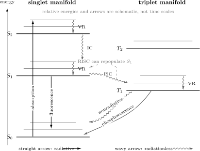
A schematic photophysical network. Straight arrows denote radiative processes; wavy arrows denote radiationless transfer or relaxation. IC is internal conversion, ISC is intersystem crossing, RISC is reverse intersystem crossing, and VR is vibrational relaxation. Relative distances, arrow lengths, and arrow order are not time scales or branching probabilities.

What the horizontal lines mean

Each bold horizontal line denotes an electronic state such as $S_0$, $S_1$, or $T_1$. Nearby thinner lines represent vibrational sublevels. The vertical spacing is only qualitative unless numerical energies are supplied.

The diagram usually suppresses:

• rotational and spin substructure;
• multidimensional nuclear coordinates;
• conical intersections and avoided crossings;
• solvent and lattice coordinates;
• conformers, aggregates, defects, and charge states;
• continua, dissociation, and chemical products;
• coherence and wavepacket phase;
• explicit photon and phonon modes.

A crossed arrow in a diagram does not calculate a rate. It asserts that a channel is being retained in the model.

What the arrows mean

Typical arrow labels are:

Symbol	Process	Photon?	Multiplicity
Absorption	Excitation by incident light	absorbed	often unchanged for E1
Fluorescence	Radiative decay	emitted	unchanged
Phosphorescence	Radiative decay	emitted	changed
VR	Vibrational relaxation within an electronic state	none	unchanged
IC	Internal conversion between electronic states	none	unchanged
ISC	Intersystem crossing	none	changed
RISC	Reverse intersystem crossing	none	changed

IUPAC defines a radiationless transition as a transition between states without photon absorption or emission. Radiationless does not mean energy disappears. Energy can enter nuclear motion, phonons, solvent modes, electronic excitations of another species, translation, or chemical products.

What the diagram does not mean

It does not imply that:

• absorption always reaches $S_2$;
• every molecule relaxes to $S_1$ before anything else happens;
• $T_1$ always lies below $S_1$;
• IC and ISC are single deterministic jumps;
• phosphorescence must be visible;
• one arrow corresponds to one exponential component;
• higher excited-state emission is impossible.

The Kasha rule is a common empirical tendency, not a diagrammatic law.

Relaxation After Excitation

Franck–Condon preparation

Electronic absorption acts rapidly compared with substantial nuclear rearrangement. It prepares a nuclear wavepacket on an excited electronic surface. Electronic Spectroscopy develops the corresponding Franck–Condon projections and distinguishes the vertical gap from a band maximum.

Immediately after the pulse, the excited ensemble may contain:

• vibrational excess energy;
• coherent superpositions of vibronic states;
• several electronic states within the pulse bandwidth;
• orientational selection by the light polarization;
• several conformers, sites, or species;
• solvent configurations inherited from the ground state.

Relaxation begins from that prepared distribution, not from a generic equilibrated $S_1$ state.

Vibrational relaxation

Vibrational relaxation redistributes energy within one electronic state and often transfers energy to a bath:

$$S_1(v'>0) \longrightarrow S_1(v'=0) + \text{bath}.$$

In an isolated molecule, intramolecular vibrational redistribution can spread energy among modes without removing it from the molecule. In solution or a solid, collisions, solvent modes, and phonons can carry it away.

Vibrational cooling can shift and reshape a time-resolved fluorescence spectrum even while the electronic population remains in $S_1$.

Internal conversion

IUPAC defines internal conversion as an isoenergetic radiationless transition between electronic states of the same multiplicity. A typical example is

$$S_2 \longrightarrow S_1^*,$$

where the asterisk indicates vibrational excitation in the receiving state. Subsequent vibrational relaxation can yield a cooled $S_1$ population.

Microscopically, internal conversion depends on vibronic coupling, energy gaps, accessible nuclear configurations, and the density of receiving states. Nonadiabatic Coupling owns that surface-dynamics description.

Intersystem crossing

IUPAC defines intersystem crossing as an isoenergetic radiationless transition between electronic states of different multiplicity. A common channel is

$$S_1 \longrightarrow T_n^*,$$

followed by triplet vibrational relaxation and internal conversion to $T_1$. Spin–orbit coupling is normally required to connect nominally pure singlet and triplet states.

Solvent and structural relaxation

The environment can reorganize around a changed excited-state charge distribution. Torsion, proton transfer, charge transfer, excimer formation, and conformational change can create a new emitting state. A time-dependent red shift or changing spectral shape can therefore report nuclear or solvent dynamics, not merely population loss.

Photochemistry and dissociation

An excited state may react, isomerize, ionize, transfer an electron, or dissociate. Such channels can lower luminescence yield without producing a simple heat-only loss. A complete branching model should name photochemical products separately from unresolved nonradiative decay whenever they are measured.

Fluorescence

Transition amplitude

For an emitting state $|e\rangle$ and lower state $|g\rangle$, the leading electric-dipole amplitude is

$$\mathbf d_{ge} = \langle g | \widehat{\mathbf d} | e \rangle.$$

In free space, the spontaneous E1 rate scales schematically as

$$k_F \propto \omega_{eg}^{3} \left| \mathbf d_{ge} \right|^2,$$

with constants and angular factors determined by conventions and environment. Einstein Coefficients gives the exact free-space relation and degeneracy bookkeeping.

The radiative rate is not solely an intrinsic molecular number. Refractive index, interfaces, cavities, photonic density of states, orientation, and nearby absorbers can modify emission. A molecule’s internal transition moment and its electromagnetic environment are separate parts of the forward model.

Why fluorescence is often prompt

For a singlet ground state and singlet excited state, the spin overlap does not suppress the E1 transition. If the electronic and vibronic transition moments are substantial, $k_F$ can compete effectively with internal conversion and intersystem crossing.

Prompt does not mean instantaneous. The observed fluorescence appears after state preparation and evolves with the emitting-state population, instrument response, and any spectral relaxation.

Fluorescence spectrum

After cooling within $S_1$, emission commonly samples

$$S_1(v'=0) \longrightarrow S_0(v'').$$

Franck–Condon factors distribute intensity among ground-state vibrational levels. The band often lies at lower photon energy than absorption because the excited ensemble relaxed before emission. The Electronic Spectroscopy page explains the 0–0 origin, Stokes shift, mirror-image approximation, and spectral-coordinate Jacobian.

Fluorescence polarization

Linearly polarized excitation preferentially selects absorbers whose absorption transition dipoles project onto the electric field. Emission can remain polarized until rotational diffusion, energy transfer, state mixing, or structural relaxation erases orientational memory.

A common steady-state anisotropy definition is

$$r = \frac{ I_{\parallel}-I_{\perp} }{ I_{\parallel}+2I_{\perp} },$$

after polarization-dependent instrument corrections. Here the subscripts refer to emission analyzed parallel and perpendicular to the excitation polarization.

Anisotropy decay is not the same as population decay. It can reveal rotation or energy migration while the total fluorescence intensity follows another time law.

Phosphorescence

Spin-forbidden does not mean impossible

For pure spin states and a spin-independent dipole operator,

$$\langle S_0 | \widehat{\mathbf d} | T_1 \rangle = 0.$$

Spin–orbit coupling mixes singlet and triplet basis states. Write

$$|\widetilde T_1\rangle \simeq |T_1\rangle + \epsilon|S_n\rangle.$$

Then

$$\begin{aligned} \langle S_0 | \widehat{\mathbf d} | \widetilde T_1 \rangle &\simeq \epsilon \langle S_0 | \widehat{\mathbf d} | S_n \rangle. \end{aligned}$$

The phosphorescence intensity borrowed through this path scales as $|\epsilon|^2$ when it is the only leading contribution. The same mixing can also enhance intersystem crossing into the triplet manifold.

The heavy-atom effect

The IUPAC heavy-atom effect is enhancement of a spin-forbidden process through stronger spin–orbit coupling from an internal or external high-$Z$ atom. It can increase ISC, phosphorescence rate, or both.

It does not guarantee brighter phosphorescence. Heavy atoms can also open nonradiative channels, alter electronic character, promote photochemistry, or increase quenching. Brightness depends on the entire rate network.

Why triplet emission is environment sensitive

A long triplet lifetime gives collisions and diffusion time to compete. Molecular oxygen is a particularly effective quencher for many triplet states. Rigid matrices, crystals, low temperature, and deoxygenation can suppress motion or collisions and make phosphorescence easier to observe.

These trends are diagnostic but not unique. Rigidity can also change electronic structure, aggregation, and phonon coupling. Oxygen can quench through energy or electron transfer and can generate reactive oxygen species.

Metastability is a rate statement

A metastable state has a small total escape rate under stated conditions. Its observed lifetime can be long because:

• the radiative transition is spin or symmetry suppressed;
• accepting vibrational or phonon states are unfavorable;
• the environment is rigid or cold;
• quenchers are absent;
• population is trapped behind a kinetic barrier.

The term does not mean the state is absolutely stable.

Spin–Orbit and Vibronic Control of ISC

A schematic golden-rule expression for intersystem crossing is

$$k_{\mathrm{ISC}} \simeq \frac{2\pi}{\hbar} \sum_f \left| \langle T_f | \widehat H_{\mathrm{SO}} | S_i \rangle \right|^2 \delta(E_f-E_i).$$

This notation compresses electronic, vibrational, and environmental degrees of freedom. A useful qualitative audit asks:

1. How large are the relevant spin–orbit matrix elements?
2. Are the singlet and triplet states close enough in energy?
3. Do vibrational modes provide overlap and symmetry coupling?
4. Is there a dense set of accepting vibronic levels?
5. Can the nuclear wavepacket reach the coupling region?
6. Do solvent, crystal, or magnetic interactions alter the states?

Orbital character as a propensity

Spin–orbit matrix elements often depend strongly on orbital character. Transitions between states with different orbital types can have larger couplings than transitions between otherwise similar states. Such El-Sayed-type statements are propensity rules, not exact selection rules. Configuration mixing, geometry, vibronic coupling, and heavy atoms can reverse a simple label-based expectation.

Reverse intersystem crossing

Triplet population can return to a singlet manifold:

$$T_1 \longrightarrow S_1.$$

This reverse intersystem crossing, RISC, can be thermally activated when $S_1$ lies moderately above $T_1$. If the repopulated $S_1$ fluoresces, the spectrum can resemble prompt fluorescence while the decay follows the slower triplet reservoir.

The energy difference

$$\Delta E_{\mathrm{ST}} = E(S_1)-E(T_1)$$

is important, but it does not determine RISC alone. Spin–orbit coupling, vibronic mediation, conformational dynamics, state density, and the environment also matter.

Minimal Rate Network

Consider a pulsed experiment that prepares $N_S(0)=N_0$ molecules in an emitting singlet state. Let

$$k_S = k_F + k_{\mathrm{IC}} + k_{\mathrm{ISC}} + k_{\mathrm{rxn}} + k_{\mathrm q} + \cdots.$$

For independent first-order channels,

$$\frac{dN_S}{dt} = -k_S N_S,$$

so

$$N_S(t) = N_0e^{-k_St}.$$

The singlet population lifetime is

$$\tau_S = \frac{1}{k_S}.$$

The prompt fluorescence photon rate before propagation and detection is

$$I_F(t) = k_F N_S(t).$$

Branching yields

Under the same model, the probability that one prepared singlet exits through channel $j$ is

$$\Phi_j = \int_0^\infty k_jN_S(t)\,dt \bigg/ N_0 = \frac{k_j}{k_S}.$$

Therefore

$$\begin{aligned} \Phi_F &= \frac{k_F}{k_S}, \\ \Phi_{\mathrm{IC}} &= \frac{k_{\mathrm{IC}}}{k_S}, \\ \Phi_{\mathrm{ISC}} &= \frac{k_{\mathrm{ISC}}}{k_S}. \end{aligned}$$

If the listed channels are exhaustive,

$$\sum_j\Phi_j=1.$$

A missing yield can indicate an omitted channel, an incorrectly counted absorbed photon, an unobserved product, or systematic calibration error.

Radiative and observed lifetimes

The fluorescence radiative lifetime for one emitting state is

$$\tau_{\mathrm{rad},F} = \frac{1}{k_F}.$$

The observed population lifetime includes every exit channel:

$$\tau_S = \frac{1}{k_S}.$$

Hence

$$\Phi_F = \frac{\tau_S}{\tau_{\mathrm{rad},F}}.$$

Equivalently,

$$k_F = \frac{\Phi_F}{\tau_S}, \qquad k_{\mathrm{other}} = \frac{1-\Phi_F}{\tau_S}.$$

The second relation yields only the sum of nonfluorescent rates. A lifetime and fluorescence yield alone cannot separate IC, ISC, transfer, reaction, and quenching.

IUPAC defines the radiative lifetime as the lifetime in the absence of radiationless transitions and discourages “natural lifetime” as an equivalent term.

Sequential singlet-to-triplet kinetics

Let triplets be formed by ISC and decay with

$$k_T = k_P + k_{\mathrm{nr},T} + k_{\mathrm q,T} + \cdots.$$

The coupled equations are

$$\begin{aligned} \frac{dN_S}{dt} &= -k_SN_S, \\ \frac{dN_T}{dt} &= k_{\mathrm{ISC}}N_S - k_TN_T. \end{aligned}$$

For $N_T(0)=0$ and $k_T\ne k_S$,

$$\begin{aligned} N_T(t) &= N_0 \frac{k_{\mathrm{ISC}}}{k_T-k_S} \\ &\quad\times \left( e^{-k_St} - e^{-k_Tt} \right). \end{aligned}$$

The phosphorescence photon rate is

$$I_P(t) = k_PN_T(t).$$

The integrated phosphorescence yield from the initially prepared singlet is

$$\Phi_P = \frac{k_{\mathrm{ISC}}}{k_S} \frac{k_P}{k_T} = \Phi_{\mathrm{ISC}} \Phi_{P|T}.$$

This factorization separates triplet formation from radiative branching out of the triplet. A weak phosphorescence yield can result from poor triplet formation, poor triplet radiative branching, or both.

Continuous weak excitation

For a constant absorbed-excitation rate $R_{\mathrm{abs}}$ in the linear regime,

$$\frac{dN_S}{dt} = R_{\mathrm{abs}} - k_SN_S.$$

The steady population is

$$N_S^{(\mathrm{ss})} = \frac{R_{\mathrm{abs}}}{k_S},$$

and the fluorescence generation rate is

$$R_F^{(\mathrm{ss})} = k_FN_S^{(\mathrm{ss})} = \Phi_FR_{\mathrm{abs}}.$$

At high excitation, ground-state depletion, excited-state absorption, annihilation, stimulated emission, heating, or photochemistry can invalidate this linear relation.

Quantum Yield

IUPAC defines a quantum yield as the number of specified events per photon absorbed. For fluorescence,

$$\Phi_F = \frac{ N_{\mathrm{fluorescence\ photons}} }{ N_{\mathrm{absorbed\ photons}} }.$$

The denominator is not the number of incident photons. Reflection, transmission, scattering, and parasitic absorption must be treated.

Event yield versus detected count

The detected number can be written schematically as

$$\begin{aligned} N_{\mathrm{det}} &= N_{\mathrm{abs}} \Phi_F \\ &\quad\times \eta_{\mathrm{geom}} \eta_{\mathrm{prop}} \eta_{\mathrm{det}}, \end{aligned}$$

where the efficiencies represent collection geometry, propagation and reabsorption, and detector response. They can depend on wavelength, polarization, position, and time.

A bright detector signal can coexist with a modest intrinsic yield if collection is excellent. A weak signal can coexist with a high yield if absorption or collection is poor.

Photon units, not raw radiant power

At wavelength $\lambda$, one photon carries energy

$$E_\gamma = \frac{hc_0}{\lambda}.$$

If a calibrated instrument reports spectral radiant power $P_\lambda$, the corresponding spectral photon rate is proportional to

$$\dot N_\lambda = \frac{ P_\lambda\lambda }{ hc_0 }.$$

Integrating uncorrected watts across wavelength does not count photons and can bias a quantum yield.

Relative and absolute measurements

A relative measurement compares integrated, response-corrected emission with a standard of known yield under matched conditions. A common dilute-solution form is

$$\begin{aligned} \Phi_x &= \Phi_r \frac{G_x}{G_r} \frac{ 1-10^{-A_r} }{ 1-10^{-A_x} } \frac{n_x^2}{n_r^2}, \end{aligned}$$

where $G$ is integrated photon-corrected emission, $A$ is absorbance at the excitation wavelength, and $n$ is refractive index. The refractive-index factor and geometry must match the calibration convention.

An integrating sphere can measure absorbed and emitted photon flux more directly, but it still requires spectral response calibration, blank subtraction, correction for reabsorption, and tests for sample change.

Quantum yield is not lifetime

Two emitters can share a lifetime but have different fluorescence yields if both radiative and nonradiative rates scale together. They can share a yield but have very different lifetimes if all rates differ by a common factor.

The pair $(\Phi_F,\tau_S)$ is more informative than either alone because, within the simple model, it gives $k_F$ and the aggregate competing rate.

Lifetimes and Decay Laws

Single-exponential population decay

For a time-independent first-order escape rate,

$$N(t) = N(0)e^{-t/\tau}.$$

If the emission spectrum and radiative rate are stationary,

$$I(t) = I(0)e^{-t/\tau}.$$

The $1/e$ time, integrated area divided by initial intensity, and maximum-likelihood exponential parameter then coincide.

When intensity does not track one population

At a fixed detection wavelength,

$$I(\lambda,t) = \sum_a k_{F,a}(\lambda,t)N_a(t).$$

Spectral relaxation, state conversion, energy transfer, multiple emitters, or time-dependent transition moments can produce rises, shifts, and nonexponential decays. One wavelength trace may not represent the total excited-state population.

Multiexponential decays

A common empirical model is

$$I(t) = \sum_{i=1}^{m} \alpha_i e^{-t/\tau_i},$$

with amplitudes $\alpha_i$ defined at the chosen time origin and detection channel.

Two averages answer different questions. The amplitude-weighted time is

$$\tau_{\mathrm{amp}} = \frac{ \displaystyle\sum_i\alpha_i\tau_i }{ \displaystyle\sum_i\alpha_i },$$

whereas the mean photon arrival time is

$$\langle t\rangle = \frac{ \displaystyle\sum_i\alpha_i\tau_i^2 }{ \displaystyle\sum_i\alpha_i\tau_i }.$$

The integrated photon fraction of component $i$ is proportional to $\alpha_i\tau_i$, not merely $\alpha_i$. A small long-lived amplitude can dominate the integrated signal.

Multiexponential fits are not unique microscopic decompositions. Continuous lifetime distributions, diffusion, transfer, spectral relaxation, and heterogeneous environments can generate similar curves.

Lifetime, coherence, and linewidth

Population relaxation time $T_1$ and optical coherence time $T_2$ obey, in a simple Markovian two-level model,

$$\frac{1}{T_2} = \frac{1}{2T_1} + \frac{1}{T_\phi},$$

where $T_\phi$ is a pure-dephasing time. Lifetime alone predicts a linewidth only when additional dephasing and inhomogeneous broadening are negligible.

For an exponential field coherence with time $T_2$, the Lorentzian full width at half maximum in ordinary frequency is

$$\Delta\nu_{\mathrm{FWHM}} = \frac{1}{\pi T_2}.$$

Line Shapes and Broadening owns the convention-sensitive derivation and non-Lorentzian limits.

Time-correlated single-photon counting

In a pulsed photon-counting experiment, the measured histogram is a convolution:

$$\begin{aligned} C_{\mathrm{obs}}(t) &= \int_{-\infty}^{\infty} R_{\mathrm{IRF}}(t') I(t-t')\,dt' \\ &\quad+ B(t), \end{aligned}$$

where $R_{\mathrm{IRF}}$ is the instrument response function and $B$ is a background model.

Deconvolution by eye is unreliable. Fit the convolved forward model and report the IRF, repetition period, time bin, fit window, background, and residuals. Count rates that are too high can produce pile-up: early photons are preferentially recorded, biasing the decay shorter.

Frequency-domain lifetime measurement

For a single exponential driven by sinusoidally modulated excitation at angular frequency $\Omega_m$, the emission has phase lag

$$\tan\phi = \Omega_m\tau$$

and modulation ratio

$$m = \frac{1}{ \sqrt{1+\Omega_m^2\tau^2} }.$$

Disagreement between phase and modulation lifetimes signals multiexponential behavior, background, or instrumental error.

Quenching

IUPAC defines quenching as nonradiative deactivation by an environmental influence or intramolecular substituent. Its distinction between dynamic and static quenching is experimentally important.

Dynamic quenching

For collisional quenching by species $Q$ with bimolecular rate constant $k_q$,

$$k_{\mathrm{tot}}([Q]) = k_0 + k_q[Q].$$

Thus

$$\tau([Q]) = \frac{1}{ k_0+k_q[Q] }.$$

With $\tau^0=1/k_0$,

$$\frac{\tau^0}{\tau} = 1+k_q\tau^0[Q].$$

If the radiative rate and absorption are unchanged, fluorescence yield and integrated intensity obey the same Stern–Volmer relation:

$$\frac{\Phi_F^0}{\Phi_F} = \frac{I_F^0}{I_F} = 1+K_{\mathrm{SV}}[Q],$$

with

$$K_{\mathrm{SV}} = k_q\tau^0.$$

Agreement between intensity and lifetime ratios supports a simple dynamic model. It does not prove one microscopic quenching mechanism.

Static quenching

Static quenching suppresses formation of the observed excited state, for example through a nonfluorescent ground-state complex. The uncomplexed fluorophores can retain their original lifetime even while total intensity falls:

$$\frac{\tau^0}{\tau} \simeq 1, \qquad \frac{I_F^0}{I_F} > 1.$$

Absorption changes, concentration dependence, and lifetime–intensity disagreement help distinguish static from dynamic behavior.

Why Stern–Volmer plots curve

Curvature can arise from:

• simultaneous static and dynamic quenching;
• multiple emissive species or sites;
• inaccessible fluorophore fractions;
• diffusion and transient encounter effects;
• quencher absorption or inner-filter artifacts;
• energy transfer, electron transfer, or reaction;
• concentration-dependent aggregation;
• changing temperature, viscosity, or refractive index.

A straight line is a model result under restrictive conditions, not a universal law.

Oxygen and triplet states

Oxygen quenching is often strongest for long-lived triplets because encounter probability accumulates over time. Deoxygenation, controlled oxygen concentration, and time-resolved measurements can therefore diagnose triplet participation.

Oxygen dependence alone is not conclusive. Oxygen can alter singlet fluorescence, react with photoproducts, change charge-transfer pathways, and participate in sensitized singlet-oxygen formation.

Delayed Fluorescence and Other Afterglow

Long-lived emission is a timing observation. The emitting transition must be identified separately.

Thermally activated delayed fluorescence

In thermally activated delayed fluorescence, TADF, triplet population reaches $S_1$ by RISC and then emits through the ordinary singlet fluorescence transition:

$$T_1 \xrightarrow{\mathrm{RISC}} S_1 \xrightarrow{k_F} S_0+h\nu.$$

The delayed spectrum can therefore resemble prompt fluorescence. Useful diagnostics include:

• delayed intensity that grows with temperature over an activated range;
• matching prompt and delayed spectral shapes after response correction;
• coupled prompt and delayed kinetics;
• oxygen sensitivity through the triplet reservoir;
• dependence on $\Delta E_{\mathrm{ST}}$ and molecular conformation.

A thermally activated trend does not by itself prove TADF; trap release and activated transport can mimic it.

Triplet–triplet annihilation

Two triplet excitations can interact:

$$T_1+T_1 \longrightarrow S_n+S_0,$$

after which the singlet may fluoresce. The rate is nonlinear:

$$\frac{dN_T}{dt} = -k_TN_T - 2k_{\mathrm{TTA}}N_T^2.$$

Delayed fluorescence from this mechanism can show excitation-power dependence, concentration dependence, diffusion sensitivity, and nonexponential kinetics. IUPAC notes that triplet–triplet annihilation is often, but not always, followed by delayed fluorescence.

Charge recombination and traps

Photoinduced charge separation can store excitation in spatially separated carriers or traps. Release and recombination later can repopulate an emitting state. The observed decay may reflect a distribution of trap depths, transport distances, and recombination rates rather than one molecular lifetime.

Diagnostics include:

• electric-field and sample-thickness dependence;
• thermoluminescence or temperature-ramp structure;
• power-law or stretched decays;
• charging history and dark-storage time;
• sample morphology and defect concentration;
• spectral evolution as different sites empty.

Mechanism table

Delayed signal	Emitting transition	Reservoir or bottleneck	Useful test
Phosphorescence	Usually $T_1\to S_0$	Slow spin-forbidden radiative decay	Spectrum, oxygen, spin–orbit perturbation
TADF	$S_1\to S_0$	Triplet population plus RISC	Temperature and prompt/delayed spectral match
TTA fluorescence	$S_n\to S_0$ after two triplets interact	Triplet density and diffusion	Excitation-power scaling
Recombination luminescence	State populated by charge recombination	Carriers or trapped charge	Electric field, dose, and trap-release tests
Persistent defect emission	Material-dependent	Traps, defects, or metastable states	Thermoluminescence and defect controls

The IUPAC delayed fluorescence entry distinguishes thermally activated, annihilation, and recombination routes.

Measuring the Network

No single experiment determines every rate. A strong analysis combines orthogonal observables.

Steady-state emission

A corrected emission spectrum gives the wavelength distribution of detected radiant or photon flux under a stated excitation. It constrains emitting states and vibronic structure but folds together preparation, yield, collection, reabsorption, and detector response.

Excitation spectrum

Scanning excitation while monitoring emission tests which absorbers feed the chosen emitting channel. Equality with absorbance requires constant quantum yield, optically thin behavior, stable sample, and proper photon-flux and detector correction.

Time-resolved emission

Prompt and delayed windows reveal population transfer, rise times, spectral relaxation, and long-lived reservoirs. A gated spectrum should report gate start, width, repetition period, and background treatment.

Absolute or relative quantum yield

Yield supplies an integrated branching probability. Combining it with a lifetime separates a radiative rate from the aggregate competing rate under the one-state first-order model.

Transient absorption and related probes

Transient absorption can detect dark singlet, triplet, charge-transfer, and product populations that do not emit strongly. Time-resolved infrared, Raman, EPR, photoelectron, and product analysis can add structural or spin specificity.

Perturbation matrix

Perturbation	Fluorescence	Phosphorescence or triplet signal	Main inference
Oxygen concentration	may decrease	often strongly decreases	collisional quenching and triplet participation
Temperature	rates and spectrum can shift	can activate RISC or nonradiative decay	barriers and thermal equilibration
Viscosity or rigidity	can suppress motion-driven loss	can enhance triplet survival	structural relaxation and collisions
Heavy-atom substitution	may decrease or shift	ISC and phosphorescence may increase	spin–orbit involvement
Excitation power	linear at low power	TTA can become nonlinear	one- versus two-excitation mechanism
Magnetic field	usually weak effect	can alter spin mixing or radical pairs	spin-correlated pathways
Concentration	reabsorption, transfer, aggregation	annihilation and quenching	intermolecular processes

Each perturbation changes more than one parameter. Use a matrix of controls, not one signature.

A Reliable Workflow

1. Define the emitted observable

State whether the measurement reports radiometric power, photon counts, corrected spectrum, gated spectrum, lifetime histogram, anisotropy, or absolute quantum yield.

2. Specify preparation

Record excitation wavelength, bandwidth, pulse duration, repetition rate, fluence, polarization, and absorbed fraction. Name every species and phase that can absorb.

3. Draw the minimal state network

Include only states and channels needed by the data, but label:

• emitting state;
• dark reservoirs;
• radiative branches;
• IC, ISC, RISC, transfer, reaction, and quenching;
• any bimolecular terms;
• the detected channel.

4. Write rate equations before fitting

Check whether the proposed network predicts a decay, rise, steady state, power law, or concentration dependence. Count independently identifiable parameter combinations.

5. Separate spectrum, lifetime, and yield

Use:

• spectrum for emitting-state and vibronic information;
• lifetime for total escape kinetics;
• yield for integrated branching;
• absorption for the prepared population;
• transient probes for dark intermediates.

6. Model the instrument

Include spectral response, IRF convolution, gate width, pile-up, background, polarization bias, collection geometry, reabsorption, and stray excitation light.

7. Apply perturbations

Vary oxygen, temperature, power, concentration, viscosity, field, isotopologue, and time window when relevant. A mechanism should predict the direction and scale of several responses.

8. Preserve uncertainty and alternatives

Report calibration uncertainty, fit covariance, model alternatives, sample history, photobleaching, and replicate variability. Do not turn one acceptable multiexponential fit into a unique microscopic state count.

Common Mistakes

Defining phosphorescence by a lifetime threshold

Phosphorescence changes spin multiplicity. Delayed fluorescence, traps, and recombination can all be long lived.

Calling all fast emission fluorescence

Fast spin-forbidden emission can occur under strong spin–orbit coupling. Timescale supports a mechanism only with spectral and state evidence.

Treating a Jablonski diagram as a measured energy landscape

It is a schematic state network. Arrow lengths are not rates, crossings are not conical intersections, and vertical spacing may not be quantitative.

Equating the radiative lifetime with the observed lifetime

The observed inverse lifetime sums radiative and nonradiative exits. Equality requires those additional rates to vanish.

Inferring separate nonradiative rates from one yield and lifetime

The pair gives $k_F$ and the sum of competing rates. It does not uniquely separate IC, ISC, reaction, transfer, and quenching.

Fitting exponentials and naming one species per term

Exponential components can arise from coupled kinetics, distributions, spectral relaxation, energy transfer, or instrument artifacts. A fit component is not automatically a molecular species.

Using incident photons in a quantum-yield denominator

Quantum yield is per absorbed photon. Reflection, transmission, and non-emissive absorbers matter.

Comparing raw emission areas in watts

Quantum yield counts photons. Correct spectral response and divide radiant energy by photon energy before integration.

Diagnosing dynamic quenching from intensity alone

Static quenching, inner-filter effects, and absorption changes can lower intensity without shortening the emitting population’s lifetime.

Assuming oxygen sensitivity proves phosphorescence

Oxygen can quench singlets, triplets, charge-transfer states, radical pairs, and photoproducts. Combine oxygen control with spectra and kinetics.

Calling delayed fluorescence phosphorescence

If a triplet reservoir repopulates $S_1$, the eventual photon is emitted by a same-multiplicity fluorescence transition even though it is delayed.

Ignoring the repetition period

Long-lived populations can survive into later excitation cycles. The measured baseline and amplitude then depend on pulse history rather than one isolated decay.

Key Takeaways

1. Fluorescence and phosphorescence are distinguished by emitting-state mechanism and spin multiplicity, not by one universal time cutoff.
2. A Jablonski diagram is a schematic state network; it does not encode rates, nuclear coordinates, or guaranteed pathways.
3. Vibrational relaxation, internal conversion, intersystem crossing, transfer, reaction, and quenching compete after excitation.
4. Under a first-order one-state model, the lifetime is the reciprocal total exit rate and each quantum yield is its channel rate divided by that total.
5. Fluorescence yield and lifetime together determine the radiative rate and aggregate competing rate, but not every nonradiative channel separately.
6. Overall phosphorescence yield factors into triplet-formation yield and radiative branching from the triplet.
7. Long-lived fluorescence can arise from RISC, triplet–triplet annihilation, or recombination and is not phosphorescence by timing alone.
8. Dynamic quenching shortens lifetime; ideal static quenching lowers intensity without changing the lifetime of uncomplexed emitters.
9. Multiexponential fits require explicit averaging conventions and do not uniquely count species.
10. Trustworthy assignments combine spectrum, lifetime, yield, dark-state probes, instrument modeling, and controlled perturbations.

Exercises

Exercise 1: Singlet branching

An emitting singlet state has

$$\begin{aligned} k_F&=8.0\times10^7\ \mathrm{s}^{-1}, \\ k_{\mathrm{IC}}&=2.0\times10^7\ \mathrm{s}^{-1}, \\ k_{\mathrm{ISC}}&=1.0\times10^7\ \mathrm{s}^{-1}. \end{aligned}$$

Assume these channels are exhaustive and first order. Find the observed lifetime, fluorescence yield, IC yield, ISC yield, and fluorescence radiative lifetime.

Solution

The total rate is

$$k_S = 1.10\times10^8\ \mathrm{s}^{-1}.$$

Therefore

$$\tau_S = \frac{1}{k_S} = 9.09\ \mathrm{ns}.$$

The branching yields are

$$\begin{aligned} \Phi_F &= \frac{8}{11} \simeq 0.727, \\ \Phi_{\mathrm{IC}} &= \frac{2}{11} \simeq 0.182, \\ \Phi_{\mathrm{ISC}} &= \frac{1}{11} \simeq 0.091. \end{aligned}$$

They sum to one. The fluorescence radiative lifetime is

$$\tau_{\mathrm{rad},F} = \frac{1}{k_F} = 12.5\ \mathrm{ns}.$$

It is longer than the observed lifetime because IC and ISC also remove singlet population.

Exercise 2: What yield and lifetime can identify

A fluorophore has $\tau_S=4.0\ \mathrm{ns}$ and $\Phi_F=0.24$. An independent triplet measurement gives $\Phi_{\mathrm{ISC}}=0.40$.

1. Find $k_S$, $k_F$, and the aggregate nonfluorescent rate.
2. Find $k_{\mathrm{ISC}}$.
3. If the only remaining channel is IC, find $k_{\mathrm{IC}}$.
4. Which rates could not be separated without the independent triplet measurement?

Solution

The total singlet escape rate is

$$k_S = \frac{1}{4.0\ \mathrm{ns}} = 2.50\times10^8\ \mathrm{s}^{-1}.$$

The fluorescence rate is

$$k_F = \Phi_Fk_S = 6.0\times10^7\ \mathrm{s}^{-1}.$$

The aggregate competing rate is

$$k_{\mathrm{other}} = (1-\Phi_F)k_S = 1.90\times10^8\ \mathrm{s}^{-1}.$$

The independent ISC yield gives

$$k_{\mathrm{ISC}} = \Phi_{\mathrm{ISC}}k_S = 1.00\times10^8\ \mathrm{s}^{-1}.$$

If IC is the only other channel,

$$\begin{aligned} k_{\mathrm{IC}} &= k_S-k_F-k_{\mathrm{ISC}} \\ &= 9.0\times10^7\ \mathrm{s}^{-1}. \end{aligned}$$

Without the triplet yield, the measured $\tau_S$ and $\Phi_F$ would determine only $k_F$ and the sum

$$k_{\mathrm{IC}} + k_{\mathrm{ISC}} + k_{\mathrm{rxn}} + \cdots.$$

They could not separate those channels.

Exercise 3: Sequential triplet formation

After a pulse, a singlet population $N_0$ decays with $k_S=1.0\times10^8\ \mathrm{s}^{-1}$ and forms triplets with $k_{\mathrm{ISC}}=2.0\times10^7\ \mathrm{s}^{-1}$. The triplet total rate is $k_T=1.0\times10^3\ \mathrm{s}^{-1}$, of which $k_P=200\ \mathrm{s}^{-1}$ is phosphorescent.

1. Find $\Phi_{\mathrm{ISC}}$.
2. Find the conditional triplet phosphorescence yield.
3. Find the overall phosphorescence yield per prepared singlet.
4. Explain the two timescales expected in $I_P(t)$.

Solution

The triplet-formation yield is

$$\Phi_{\mathrm{ISC}} = \frac{k_{\mathrm{ISC}}}{k_S} = 0.20.$$

Once a triplet exists, its phosphorescence branching probability is

$$\Phi_{P|T} = \frac{k_P}{k_T} = 0.20.$$

Thus

$$\Phi_P = \Phi_{\mathrm{ISC}}\Phi_{P|T} = 0.040.$$

The triplet population is

$$\begin{aligned} N_T(t) &= N_0 \frac{k_{\mathrm{ISC}}}{k_T-k_S} \\ &\quad\times \left( e^{-k_St} - e^{-k_Tt} \right). \end{aligned}$$

It rises on the singlet time scale

$$\tau_S=10\ \mathrm{ns}$$

and decays on the triplet time scale

$$\tau_T=1.0\ \mathrm{ms}.$$

Because these scales are widely separated, an instrument with nanosecond resolution sees rapid triplet formation followed by millisecond phosphorescence decay.

Exercise 4: Dynamic versus static quenching

An unquenched fluorophore has $\tau^0=5.0\ \mathrm{ns}$. A quencher has $k_q=2.0\times10^9\ \mathrm{M}^{-1}\mathrm{s}^{-1}$ and concentration $[Q]=0.020\ \mathrm{M}$.

1. Predict $\tau^0/\tau$ for pure dynamic quenching.
2. Find the quenched lifetime.
3. Predict $\Phi_F^0/\Phi_F$.
4. What observation would instead suggest a dominant static component?

Solution

The Stern–Volmer constant is

$$\begin{aligned} K_{\mathrm{SV}} &= k_q\tau^0 \\ &= \left( 2.0\times10^9 \right) \left( 5.0\times10^{-9} \right) \\ &= 10\ \mathrm{M}^{-1}. \end{aligned}$$

Thus

$$\frac{\tau^0}{\tau} = 1+K_{\mathrm{SV}}[Q] = 1.20.$$

The lifetime is

$$\tau = \frac{5.0\ \mathrm{ns}}{1.20} = 4.17\ \mathrm{ns}.$$

For ideal dynamic quenching,

$$\frac{\Phi_F^0}{\Phi_F} = 1.20.$$

If integrated intensity or yield decreased while the lifetime of the remaining fluorescent population stayed near $5.0\ \mathrm{ns}$, static quenching, an inner-filter artifact, or inhibited excited-state formation would be more plausible than pure dynamic quenching.

Exercise 5: Two lifetime averages

A decay is fitted by

$$I(t) = 0.70e^{-t/(2.0\ \mathrm{ns})} + 0.30e^{-t/(8.0\ \mathrm{ns})}.$$

Find:

1. the amplitude-weighted lifetime;
2. the mean photon arrival time;
3. the integrated photon fraction from the $8.0\ \mathrm{ns}$ component.

Solution

The amplitudes sum to one, so

$$\begin{aligned} \tau_{\mathrm{amp}} &= 0.70(2.0) + 0.30(8.0) \\ &= 3.8\ \mathrm{ns}. \end{aligned}$$

The mean photon arrival time is

$$\begin{aligned} \langle t\rangle &= \frac{ 0.70(2.0)^2+0.30(8.0)^2 }{ 0.70(2.0)+0.30(8.0) } \\ &= \frac{22.0}{3.8}\ \mathrm{ns} \\ &\simeq 5.79\ \mathrm{ns}. \end{aligned}$$

The integrated areas are proportional to

$$\alpha_1\tau_1=1.4, \qquad \alpha_2\tau_2=2.4.$$

Therefore the long component contributes

$$\frac{2.4}{1.4+2.4} \simeq 0.632,$$

or about $63.2\%$ of the photons, even though its time-zero amplitude is only $30\%$.

Exercise 6: Lifetime-limited coherence

An optical transition has population lifetime $T_1=10\ \mathrm{ns}$.

1. If pure dephasing is absent, find $T_2$ and the lifetime-limited Lorentzian FWHM in hertz.
2. If the measured coherence time is instead $T_2=2.0\ \mathrm{ns}$, find $1/T_\phi$.

Solution

Without pure dephasing,

$$\frac{1}{T_2} = \frac{1}{2T_1},$$

so

$$T_2 = 2T_1 = 20\ \mathrm{ns}.$$

The FWHM is

$$\begin{aligned} \Delta\nu_{\mathrm{FWHM}} &= \frac{1}{\pi T_2} \\ &= \frac{1}{ \pi(20\times10^{-9}\ \mathrm s) } \\ &\simeq 15.9\ \mathrm{MHz}. \end{aligned}$$

For the measured $T_2=2.0\ \mathrm{ns}$,

$$\begin{aligned} \frac{1}{T_\phi} &= \frac{1}{T_2} - \frac{1}{2T_1} \\ &= 5.0\times10^8 - 5.0\times10^7 \\ &= 4.5\times10^8\ \mathrm{s}^{-1}. \end{aligned}$$

The line is therefore far from lifetime limited.

Exercise 7: Diagnose delayed emission

A material has prompt emission centered at $520\ \mathrm{nm}$ and a delayed component with the same corrected spectral shape. The delayed intensity increases from $200$ to $300\ \mathrm K$, is suppressed by oxygen, and becomes superlinear in excitation power at high fluence.

Which mechanisms are supported? Which additional measurements would distinguish TADF from triplet–triplet annihilation?

Solution

The matching spectrum indicates that prompt and delayed photons may be emitted from the same singlet state. This disfavors assigning the delayed component to a spectrally distinct phosphorescence transition, but does not exclude an overlapping spectrum.

Increasing delayed intensity with temperature supports an activated route such as RISC and therefore TADF. Oxygen suppression supports a triplet reservoir. Superlinear power dependence at high fluence supports a bimolecular contribution such as triplet–triplet annihilation. The data may contain both mechanisms.

Useful tests are:

• delayed intensity and lifetime versus excitation fluence over several decades;
• temperature-dependent prompt and delayed amplitudes in the low-fluence limit;
• concentration and viscosity dependence;
• direct triplet transient absorption;
• magnetic-field effects where relevant;
• global fitting to coupled $S_1$–$T_1$ kinetics including a quadratic triplet term;
• repetition-rate dependence to test triplet accumulation.

TADF can remain first order in the low-excitation regime, whereas TTA requires two triplets and becomes density dependent.

Exercise 8: Audit a brightening claim

Adding a heavy-atom substituent shortens a molecule’s measured emission lifetime from $8.0$ to $1.0\ \mathrm{ns}$ and lowers its fluorescence yield from $0.80$ to $0.05$. A delayed red emission also appears.

1. Compute the original and substituted fluorescence rates.
2. Compute the aggregate competing rates.
3. Does the result prove that spin–orbit coupling increased?
4. List measurements needed to identify the delayed band.

Solution

For the original molecule,

$$\begin{aligned} k_F &= \frac{0.80}{8.0\ \mathrm{ns}} = 1.0\times10^8\ \mathrm{s}^{-1}, \\ k_{\mathrm{other}} &= \frac{0.20}{8.0\ \mathrm{ns}} = 2.5\times10^7\ \mathrm{s}^{-1}. \end{aligned}$$

For the substituted molecule,

$$\begin{aligned} k_F' &= \frac{0.05}{1.0\ \mathrm{ns}} = 5.0\times10^7\ \mathrm{s}^{-1}, \\ k_{\mathrm{other}}' &= \frac{0.95}{1.0\ \mathrm{ns}} = 9.5\times10^8\ \mathrm{s}^{-1}. \end{aligned}$$

The substitution greatly increases aggregate nonfluorescent decay and also changes the fluorescence rate. This is consistent with a heavy-atom effect opening ISC, but the two measurements do not isolate ISC from internal conversion, reaction, transfer, or quenching.

To identify the delayed red band, measure:

• its time-resolved spectrum and lifetime;
• triplet yield by transient absorption or sensitization;
• oxygen dependence;
• temperature dependence;
• magnetic-field or spin-resonance response where feasible;
• absolute phosphorescence and fluorescence yields;
• excitation spectrum and power dependence;
• photoproduct and aggregation controls.

A delayed band with a different spectrum, strong oxygen sensitivity, and triplet-state correlation would support phosphorescence, but the assignment requires the combined evidence.

Further Connections

• Einstein Coefficient Reference separates channel $A$ values, radiative lifetime, observed lifetime, branching fractions, and quantum yield.
• Electronic Spectroscopy connects absorption preparation, vibronic structure, 0–0 energies, and fluorescence spectra.
• Transition Rates develops golden-rule rates, competing channels, and continuum normalization.
• Einstein Coefficients defines spontaneous and stimulated radiative coefficients.
• Absorption and Emission develops emissivity, radiative transfer, optical depth, and detected power.
• Oscillator Strengths connects absorption strength to transition moments and radiative data.
• Line Shapes and Broadening separates population decay, coherence decay, inhomogeneity, and instrument response.
• Selection Rules in Spectroscopy classifies exact, approximate, and propensity rules.
• Nonadiabatic Coupling develops internal conversion and multistate nuclear dynamics.
• Conical Intersections develops important molecular funnels for ultrafast nonradiative decay.
• Pauli Rate Equations owns classical population kinetics derived from open-system models.
• Lindblad–GKSL Equation owns completely positive Markovian quantum dynamics.
• Amplitude-Damping Master Equation develops population relaxation and coherence decay for a quantum transition.
• Quantum-Jump Trajectories connects emission channels to conditioned photon records.
• Cavity QED develops environment-modified spontaneous emission and Purcell physics.

References

• IUPAC, “fluorescence,” Compendium of Chemical Terminology, 5th ed. — phenomenological fluorescence definition.
• IUPAC, “phosphorescence,” Compendium of Chemical Terminology, 5th ed. — phenomenological and spin-multiplicity definitions.
• IUPAC, “Jablonski diagram,” Compendium of Chemical Terminology, 5th ed. — state-diagram conventions and arrow meanings.
• IUPAC, “internal conversion,” Compendium of Chemical Terminology, 5th ed. and “intersystem crossing” — radiationless same- and different-multiplicity transitions.
• IUPAC, “quantum yield,” Compendium of Chemical Terminology, 5th ed. and “radiative lifetime” — event-count and lifetime conventions.
• IUPAC, “quenching,” Compendium of Chemical Terminology, 5th ed. and “Stern–Volmer kinetic relationships” — dynamic and static quenching terminology and kinetics.
• S. E. Braslavsky, “Glossary of Terms Used in Photochemistry, 3rd Edition,” Pure and Applied Chemistry 79, 293–465 (2007) — authoritative photochemical nomenclature and measurement definitions.
• J. R. Lakowicz, Principles of Fluorescence Spectroscopy, 3rd ed., Springer, 2006 — fluorescence spectra, anisotropy, lifetimes, yields, quenching, and instrumentation.
• B. Valeur and M. N. Berberan-Santos, Molecular Fluorescence: Principles and Applications, 2nd ed., Wiley-VCH, 2012 — molecular photophysics from state preparation through time-resolved measurements.
• N. J. Turro, V. Ramamurthy, and J. C. Scaiano, Modern Molecular Photochemistry of Organic Molecules, University Science Books, 2010 — singlet and triplet photochemistry, energy transfer, and reaction pathways.
• J. B. Birks, Photophysics of Aromatic Molecules, Wiley-Interscience, 1970 — foundational rate, fluorescence, phosphorescence, and delayed fluorescence treatment.
• M. Kasha, “Characterization of Electronic Transitions in Complex Molecules,” Discussions of the Faraday Society 9, 14–19 (1950), doi:10.1039/DF9500900014 — origin of the rule concerning emission from the lowest state of a multiplicity.
• M. A. El-Sayed, “Spin–Orbit Coupling and the Radiationless Processes in Nitrogen Heterocyclics,” Journal of Chemical Physics 38, 2834–2838 (1963), doi:10.1063/1.1733610 — orbital-character propensity for intersystem crossing.