Ultrafast Spectroscopy Overview

Ultrafast spectroscopy uses controlled short pulses and phase-sensitive detection to infer how quantum systems evolve on femtosecond and attosecond timescales. A first interaction prepares a non-equilibrium state. The system evolves for a controlled delay. A later interaction converts some feature of that state into an observable such as transmitted light, fluorescence, photoelectrons, ions, X-rays, or diffracted particles.

The essential inference chain is

$$\begin{gathered} \text{characterized pulses} \\ \downarrow \\ \text{prepared density operator} \\ \downarrow \\ \text{coherent and dissipative evolution} \\ \downarrow \\ \text{probe-dependent signal} \\ \downarrow \\ \text{dynamical model and parameters}. \end{gathered}$$

The delay coordinate is experimentally precise, but it is not automatically a direct movie time. Each data point is an ensemble measurement filtered by the pump, probe, detector, sample response, and data processing. Calling a delay trace a “molecular movie” is justified only after the mapping from quantum dynamics to signal has been established.

Canonical Scope

This page is a gateway to time-resolved spectroscopy. It develops:

• pulse duration, bandwidth, spectral phase, chirp, and pulse characterization;
• preparation of electronic and vibrational wave packets;
• pump–probe timing and the instrument response function;
• population, coherence, dephasing, and relaxation signatures;
• common optical, photoelectron, and multidimensional observables;
• the distinct but overlapping femtosecond and attosecond regimes;
• a reproducible workflow for assigning dynamical mechanisms.

Neighboring pages own the underlying derivations:

• Fourier Transform owns the transform conventions and time–frequency mathematics.
• Resonant Driving develops finite-pulse transition amplitudes and coherent accumulation.
• Line Shapes and Broadening owns homogeneous, inhomogeneous, and instrumental spectral widths.
• Nonadiabatic Coupling owns coupled electronic–nuclear dynamics and surface-hopping caveats.
• Conical Intersections owns branching-plane geometry, Berry phase, and photochemical funnels.
• Dephasing vs Dissipation owns the open-system distinction between coherence loss and energy relaxation.
• Correlation Functions Overview owns equilibrium and non-equilibrium response language used in condensed matter.
• Pump–Probe Spectroscopy owns absorbed-fluence, depth-profile, transient-reflectivity, trARPES, coherent-phonon, and light-induced-state practice in quantum materials.

The present page connects those subjects to actual delay-dependent measurements. It does not replace full treatments of nonlinear optics, multidimensional spectroscopy, high-harmonic generation, or ultrafast electron and X-ray scattering.

What Time-Resolved Spectroscopy Measures

Repeated preparation, not one evolving specimen

Most pump–probe experiments repeat a cycle:

1. prepare a nominally identical sample or allow it to return to its initial state;
2. apply a pump pulse;
3. wait for a controlled delay $\tau$;
4. apply a probe pulse;
5. record one or more detector channels;
6. change $\tau$ and repeat.

The assembled trace is stroboscopic. Its interpretation assumes that the initial ensemble, pulse sequence, and environment are reproducible. At high repetition rate, incomplete recovery, sample heating, photochemistry, charge accumulation, or flow can violate that assumption.

An idealized signal is

$$S(\tau) = \operatorname{Tr} \left[ W_{\mathrm{pr}}\rho(\tau) \right],$$

where $\rho(\tau)$ is the state just before the probe and $W_{\mathrm{pr}}$ is a probe-and-detection window operator. Two probes with different photon energies, polarizations, ionization channels, or collection geometries generally have different $W_{\mathrm{pr}}$ and therefore record different traces from the same underlying state.

A method family

Method	Recorded observable	Typical inference	Important caveat
Transient absorption	Pump-induced transmission or absorbance change versus probe energy and delay	Populations, stimulated emission, excited-state absorption, spectral shifts	Several pathways overlap with signs and phases
Time-resolved fluorescence	Photon counts, spectrum, polarization, or arrival time	Emissive-state population and relaxation	Dark states and nonradiative pathways can be invisible
Time-resolved photoelectron spectroscopy	Electron energy, angle, spin, or coincidence channel	Ionization-accessible electronic and nuclear dynamics	Ionization matrix elements and ionic final states gate the signal
Time-resolved Raman spectroscopy	Raman shift and intensity versus delay	Vibrational structure and evolving local environment	Resonance enhancement and pulse overlap can reshape intensity
Two-dimensional spectroscopy	Correlation between excitation and detection frequencies	Couplings, inhomogeneity, transfer, and coherence pathways	Phase stability and pathway separation are essential
Ultrafast diffraction	Momentum-resolved electron or X-ray scattering	Pair distributions and structural change	Inversion to geometry is incomplete and model dependent

“Ultrafast” names the temporal scale, not a single interaction or detector. The observable must be stated before a decay or oscillation is assigned.

Ultrashort Pulses

Envelope, carrier, and spectrum

A real electric field can be represented by a positive-frequency component,

$$E^{(+)}(t) = \frac12 \mathcal E(t)e^{-i\omega_ct},$$

plus its complex conjugate. The carrier frequency is $\omega_c$ and the complex envelope $\mathcal E(t)$ contains the pulse amplitude and phase. A Fourier convention is

$$\widetilde E^{(+)}(\omega) = \int_{-\infty}^{\infty} E^{(+)}(t)e^{i\omega t}\,dt.$$

The spectral intensity is proportional to $|\widetilde E^{(+)}(\omega)|^2$, but intensity alone does not specify the time-domain pulse. Write

$$\widetilde E^{(+)}(\omega) = \left| \widetilde E^{(+)}(\omega) \right| e^{i\phi(\omega)}.$$

The spectral phase may be expanded near $\omega_c$:

$$\begin{aligned} \phi(\omega) ={}& \phi_0 + \phi_1(\omega-\omega_c) \\ &+ \frac{\phi_2}{2} (\omega-\omega_c)^2 \,+\cdots . \end{aligned}$$

$\phi_0$ contains a carrier phase, $\phi_1$ shifts the pulse arrival time, and $\phi_2$ is group-delay dispersion that produces linear chirp. Higher orders create more complicated temporal structure. A broad spectrum can therefore support a short pulse without actually being compressed to that duration.

Gaussian time–bandwidth product

For a transform-limited Gaussian intensity pulse with temporal FWHM $\Delta t$,

$$I(t) = I_0 \exp\left[ -4\ln2 \left( \frac{t}{\Delta t} \right)^2 \right].$$

Its intensity spectrum is also Gaussian, and the frequency FWHM obeys

$$\Delta\nu\,\Delta t = \frac{2\ln2}{\pi} \simeq 0.441.$$

Equivalently,

$$\Delta E = h\Delta\nu \simeq \frac{0.441h}{\Delta t}.$$

This is not a universal numerical uncertainty relation. The constant changes with pulse shape and with whether widths refer to field amplitude, intensity, RMS width, or FWHM. For example, a transform-limited $\operatorname{sech}^2$ intensity pulse has $\Delta\nu\Delta t\simeq0.315$.

The time–bandwidth product is a lower bound for a specified pulse shape. A measured product larger than the transform limit can arise from chirp, satellite pulses, spatiotemporal coupling, or inconsistent width definitions.

Duration and selectivity trade off

A $20\ \mathrm{fs}$ transform-limited Gaussian pulse has

$$\begin{aligned} \Delta\nu &= \frac{0.441}{20\ \mathrm{fs}} \\ &\simeq 22.1\ \mathrm{THz}, \end{aligned}$$

and therefore

$$\Delta E\simeq0.0912\ \mathrm{eV}.$$

Its wavenumber bandwidth is about $736\ \mathrm{cm^{-1}}$. Such a pulse can resolve rapid motion in time while exciting many nearby vibronic transitions. A long narrowband pulse provides better spectral selectivity but poorer direct timing. Multidimensional and pulse-shaping methods recover some frequency selectivity through controlled coherence intervals; they do not repeal Fourier relations.

Pulse duration must be measured

An optical intensity autocorrelation does not uniquely reconstruct a pulse. It requires an assumed shape and contains no complete spectral-phase information. Methods such as frequency-resolved optical gating (FROG) and spectral-phase interferometry for direct electric-field reconstruction (SPIDER) retrieve or constrain both amplitude and phase under stated assumptions.

For credible ultrafast work, pulse characterization should be performed:

• at or near the sample, not only at the laser output;
• across the relevant beam profile when spatial chirp may matter;
• over the wavelength range used by pump and probe;
• with sample cells, windows, objectives, and air paths included;
• at representative pulse energy, since nonlinear compression can be energy dependent.

The pulse arriving at the sample is part of the experiment, not merely a nominal specification from the source.

Pulses Prepare Wave Packets

Coherent excitation of several eigenstates

In weak first-order excitation from $|g\rangle$, the amplitude for an eigenstate $|n\rangle$ contains the spectral field at its transition frequency:

$$c_n \propto -\frac{i}{\hbar} \langle n| \boldsymbol{\mu}\cdot\boldsymbol{\epsilon} |g\rangle \widetilde E^{(+)}(\omega_{ng}).$$

A narrowband pulse may select one eigenstate. A broadband phase-coherent pulse can prepare

$$|\psi(0^+)\rangle = \sum_n c_n|n\rangle.$$

Subsequent closed evolution gives

$$|\psi(t)\rangle = \sum_n c_n e^{-iE_nt/\hbar}|n\rangle.$$

For an observable $A$,

$$\begin{aligned} \langle A\rangle_t ={}& \sum_{m,n} c_m^*c_n \\ &\times e^{-i(E_n-E_m)t/\hbar} A_{mn}. \end{aligned}$$

The diagonal terms carry populations. Off-diagonal terms produce quantum beats when the observable and probe retain sensitivity to their relative phase.

Density-operator form

For an ensemble,

$$\rho_{mn}(t) = \rho_{mn}(0) e^{-i\omega_{mn}t} e^{-g_{mn}(t)}.$$

$g_{mn}(t)$ summarizes dephasing in a chosen model. It need not be linear in $t$; static Gaussian disorder, Markovian phase noise, spectral diffusion, and non-Markovian environments produce different functions.

A pump pulse can create simultaneously:

• excited-state populations $\rho_{nn}$;
• electronic coherences between electronic eigenstates;
• vibrational coherences within one electronic manifold;
• vibronic coherences involving mixed electronic and nuclear character;
• orientational anisotropy in an ensemble;
• spatial gratings or other collective optical coherences.

A measured oscillation does not identify which category is present. Its frequency, phase, polarization dependence, excitation spectrum, temperature dependence, isotope dependence, and dephasing must all be tested.

Nuclear wave packets

In a molecular adiabatic expansion,

$$\Psi(\mathbf r,\mathbf R,t) = \sum_a \chi_a(\mathbf R,t) \phi_a(\mathbf r;\mathbf R).$$

A short electronic excitation acts over a nuclear configuration distribution and prepares one or more nuclear wave packets $\chi_a(\mathbf R,0^+)$. Their evolution can include:

• motion on anharmonic potential-energy surfaces;
• dispersion and revivals;
• branching into different nuclear regions;
• nonadiabatic transfer between electronic surfaces;
• entanglement between electronic and nuclear degrees of freedom;
• environmental decoherence and relaxation.

A localized wave packet can resemble a classical packet for some observables and times, but it is not a point following one trajectory. Wave Packets develops the general superposition language.

Pump–Probe Logic

The IUPAC pump–probe definition emphasizes a strong pump that initiates a process and a delayed weaker probe that monitors an optical property. Modern experiments extend the same logic to XUV, X-ray, photoelectron, ion, electron-diffraction, and other probes.

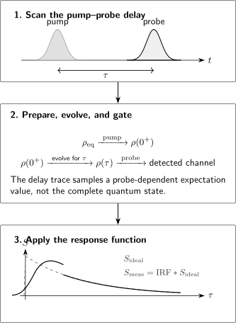
Changing the pump–probe delay $\tau$ samples a probe-dependent signal from $\rho(\tau)$. The measured transient is broadened and sometimes distorted by the instrument response function (IRF), so delay resolution is not set by one nominal pulse width.

Differential absorption

For a transmission experiment, one common convention is

$$\Delta A(\omega,\tau) = -\log_{10} \left[ \frac{ I_{\mathrm{pump\ on}}(\omega,\tau) }{ I_{\mathrm{pump\ off}}(\omega) } \right].$$

Positive $\Delta A$ means less transmitted probe under this convention; negative $\Delta A$ means more. Other communities report $\Delta T/T$, $\Delta R/R$, optical density, or a heterodyne field with different signs. The displayed color map is uninterpretable until the definition and phase convention are known.

In a common electronic transient-absorption picture, three contributions are often discussed:

1. Ground-state bleach: pump depletion reduces ground-state absorption.
2. Stimulated emission: the probe stimulates emission from an excited state.
3. Excited-state absorption: the probe promotes the prepared system to a higher state.

Bleach and stimulated emission often appear with the same sign in $\Delta A$, while excited-state absorption often has the opposite sign. This is not a universal assignment rule. Overlapping bands, refractive signals, coherent pathways, scattering, heating, and population-dependent line shifts can reverse or mix apparent features.

Pump–probe is nonlinear response

In weak optical pump–probe spectroscopy, two pump field interactions prepare a population or coherence and a probe interaction generates a third-order polarization. Schematically,

$$\begin{aligned} P^{(3)}(t) ={}& \int_0^\infty dt_3 \int_0^\infty dt_2 \int_0^\infty dt_1 \\ &\times R^{(3)}(t_3,t_2,t_1) \\ &\times E_3(t-t_3) \\ &\times E_2(t-t_3-t_2) \\ &\times E_1(t-t_3-t_2-t_1). \end{aligned}$$

$R^{(3)}$ contains nested commutators and propagators of the material system. Distinct Liouville-space pathways can reach the same detected frequency and interfere. The delay trace is therefore not generally equal to one excited-state population.

The Linear Response Preview introduces response functions. Full nonlinear-response and multidimensional derivations belong to specialist treatments.

Pulse overlap and time zero

Near zero delay, pump and probe overlap in the sample. The signal can contain coherent artifacts, cross-phase modulation, four-wave mixing, two-photon absorption, or pump-induced probe reshaping. These terms may be useful, but they are not automatically an ultrafast population rise.

Time zero can depend on:

• probe wavelength because of dispersion;
• sample position and thickness;
• beam angle and pulse-front tilt;
• nonlinear crystal or reference material;
• data-processing and phase conventions.

A broadband probe may therefore require a wavelength-dependent time-zero correction. Applying an empirical correction without reporting it can manufacture or erase apparent dynamics.

Instrument Response

Convolution

A common model is

$$S_{\mathrm{meas}}(\tau) = \int_{-\infty}^{\infty} G_{\mathrm{IRF}}(\tau-\tau') S_{\mathrm{ideal}}(\tau')\,d\tau'.$$

$G_{\mathrm{IRF}}$ includes pump and probe envelopes, timing jitter, detector response, group-velocity mismatch, and any additional gate. If the relevant contributions are independent Gaussians with FWHM values $\Delta t_j$, then

$$\Delta t_{\mathrm{IRF}} = \sqrt{ \sum_j (\Delta t_j)^2 }.$$

For a $35\ \mathrm{fs}$ pump, $50\ \mathrm{fs}$ probe, and $20\ \mathrm{fs}$ timing-jitter width, all expressed as Gaussian FWHM values,

$$\begin{aligned} \Delta t_{\mathrm{IRF}} &= \sqrt{ (35\ \mathrm{fs})^2 + (50\ \mathrm{fs})^2 + (20\ \mathrm{fs})^2 } \\ &\simeq 64.2\ \mathrm{fs}. \end{aligned}$$

Mixing RMS and FWHM widths in this quadrature rule is a common numerical error.

Deconvolution is an inference

If an observed rise is comparable to the IRF, the intrinsic timescale is not read directly from the graph. It must be inferred from a forward fit. Deconvolution can be ill-conditioned, especially when:

• the IRF is uncertain or non-Gaussian;
• time zero drifts;
• several kinetic components overlap;
• coherent artifacts contribute;
• the signal has wavelength-dependent response;
• the assumed kinetic model is too restrictive.

A fit can estimate a timescale shorter than the nominal IRF when the signal-to-noise ratio and response calibration are strong, but the uncertainty and model dependence increase. “Sub-IRF” does not mean impossible; it does mean that visual resolution and parameter inference must not be confused.

Sampling is not resolution

A delay step of $1\ \mathrm{fs}$ does not create $1\ \mathrm{fs}$ temporal resolution. It samples a signal already blurred by the pulses and instrument. Conversely, coarse sampling can alias oscillations even when the pulses are short enough to excite and detect them.

If a beat has angular frequency $\Omega_b$, the delay sampling interval should satisfy a Nyquist condition,

$$\Delta\tau < \frac{\pi}{\Omega_b},$$

with a practical margin for fitting phase and damping. The total scan window sets frequency resolution in a delay-axis Fourier transform.

Coherence and Dephasing

Populations and coherences

In a basis of energy eigenstates:

$$P_n(t)=\rho_{nn}(t)$$

is a population, while

$$\rho_{mn}(t), \qquad m\ne n,$$

is a coherence. A population can decay without oscillating. A coherence usually carries a phase at $\omega_{mn}$ and can generate beats if the probe couples the interfering pathways to the same detector outcome.

Coherence is basis dependent. Electronic coherence in an adiabatic basis can be represented differently in a diabatic basis, while measurable signals remain invariant when states, operators, and dynamics are transformed consistently.

Ensemble dephasing

Suppose members of an ensemble have static frequency offsets $\delta\omega$. The ensemble coherence contains

$$\Phi(t) = \left\langle e^{-i\delta\omega t} \right\rangle.$$

For a Gaussian offset distribution with standard deviation $\sigma_\omega$,

$$\Phi(t) = \exp\left( -\frac{\sigma_\omega^2t^2}{2} \right).$$

For a Lorentzian offset distribution with HWHM $\Gamma$, it is

$$\Phi(t)=e^{-\Gamma|t|}.$$

Thus a fitted exponential is not proof of Markovian environmental dephasing, and a Gaussian decay is not automatically instrumental. Echo and rephasing methods can separate some reversible inhomogeneity from irreversible phase loss.

Population relaxation also destroys coherence

For a simple Markovian two-level model,

$$\frac{1}{T_2} = \frac{1}{2T_1} + \frac{1}{T_\phi}.$$

Ultrafast experiments often involve multilevel manifolds, spectral diffusion, non-exponential kinetics, and evolving bases, so this relation must not be applied mechanically to every beat envelope. The same caution is developed in Dephasing vs Dissipation.

Assigning an oscillation

A credible oscillation assignment tests:

1. frequency against known vibrational, excitonic, spin, or electronic splittings;
2. phase across detection energy and polarization;
3. pump-spectrum and probe-window dependence;
4. isotope, temperature, solvent, orientation, or field dependence;
5. persistence outside pulse overlap;
6. robustness to background and kinetic-model choices;
7. agreement with a response calculation, not only a Fourier peak.

Impulsive Raman excitation can create ground-state vibrational coherence that appears in the same spectral region as excited-state wave-packet motion. A beat is evidence for interference; its physical location requires additional controls.

Molecular Dynamics

Vertical preparation and subsequent motion

The Franck–Condon picture says that an electronic transition samples the initial nuclear wavefunction before substantial nuclear motion during the optical interaction. After the pulse, the prepared nuclear wave packet evolves on one or more electronic surfaces.

The sequence is conceptually

$$\begin{gathered} \text{ground-state nuclear distribution} \\ \xrightarrow{\ \text{pump}\ } \\ \text{excited vibronic wave packet} \\ \xrightarrow{\ \substack{\text{Hamiltonian}\\\text{and environment}}\ } \\ \begin{array}{c} \text{motion, branching, transfer,}\\[-0.15em] \text{and relaxation} \end{array}. \end{gathered}$$

Pulse duration, bandwidth, and transition dipoles determine the initial wave packet. Potential surfaces and derivative couplings determine its closed-system evolution. Solvent, phonons, collisions, and radiation add open-system dynamics.

Probe windows convert motion into signal

Suppose a probe ionizes only where an ionic potential surface is accessible. Then the photoelectron yield can peak when a nuclear wave packet enters that geometry region. A different probe photon energy can define a different window and shift or remove the peak without changing the underlying dynamics.

Likewise:

• transient absorption follows energy gaps and transition dipoles that evolve with nuclear configuration;
• fluorescence follows emissive states and radiative selection;
• diffraction weights pair correlations and scattering factors;
• photoelectron angular distributions weight continuum partial waves;
• ion fragments weight dissociation and detection efficiencies.

Geometry is therefore inferred by comparing multiple observables with a forward dynamical model. One spectral maximum is not a Cartesian coordinate.

Nonadiabatic dynamics

Near an avoided crossing or conical intersection, electronic and nuclear motions cannot be separated into one wave packet on one fixed surface. Population can branch, electronic coherence can be created or lost, and the probe can mix signals from several electronic characters.

Nonadiabatic Coupling develops derivative couplings and dynamics methods. Conical Intersections explains why one optimized minimum-energy intersection is not itself a time-resolved mechanism.

Ultrafast data can constrain access times, branching, and product formation, but only a global fit across detection channels can distinguish a crossing time from wave-packet arrival at a probe window.

Femtosecond Regime

One femtosecond is

$$1\ \mathrm{fs}=10^{-15}\ \mathrm s.$$

Femtosecond pulses overlap many molecular and condensed-matter timescales:

Process	Illustrative scale	Qualification
Electronic dephasing and charge redistribution	few femtoseconds to hundreds of femtoseconds	Strongly system and environment dependent
Molecular vibration	roughly $10$–$1000\ \mathrm{fs}$ periods	Light-atom stretches are faster than torsions and collective modes
Internal conversion and intersystem crossing	femtoseconds to nanoseconds	Coupling, energy gaps, and density of states matter
Solvation and dielectric response	tens of femtoseconds to many picoseconds	Often multicomponent and solvent specific
Energy and charge transfer	femtoseconds to nanoseconds	Coherent and incoherent regimes can coexist
Bond rearrangement and fragmentation	tens of femtoseconds onward	Detection may occur long after decisive branching

These ranges overlap. “Electronic is fast, nuclear is slow” is a useful scale-separation intuition, not a universal assignment rule.

Femtochemistry

Femtochemistry established that pump–probe observables can follow molecular wave packets through regions connecting reactants and products. The central advance was dynamical timing, not direct observation of a classical transition-state structure in every experiment.

Modern femtosecond spectroscopy can combine:

• broadband transient absorption for electronic populations and spectral evolution;
• fluorescence up-conversion for emissive-state dynamics;
• time-resolved photoelectron spectra for coupled electronic–nuclear channels;
• femtosecond stimulated Raman or time-resolved infrared spectra for vibrational structure;
• multidimensional spectra for couplings and inhomogeneity;
• ultrafast diffraction and X-ray spectroscopy for structural and element-specific information.

The strongest mechanistic conclusions use complementary windows rather than one trace.

Attosecond Regime

One attosecond is

$$1\ \mathrm{as}=10^{-18}\ \mathrm s.$$

Sub-femtosecond pulses require very broad coherent bandwidth. A $200\ \mathrm{as}$ transform-limited Gaussian pulse has

$$\begin{aligned} \Delta\nu &\simeq \frac{0.441}{200\ \mathrm{as}} \\ &\simeq 2.21\ \mathrm{PHz}, \end{aligned}$$

corresponding to

$$\Delta E\simeq9.12\ \mathrm{eV}.$$

Extreme-ultraviolet (XUV) and soft-X-ray attosecond pulses are commonly generated through high-harmonic processes and synchronized to a strong infrared field. Their bandwidth can ionize several channels at once, making continuum phases and channel coupling part of the measurement.

Attosecond streaking

In a simplified streaking picture, an XUV pulse releases an electron and a synchronized infrared field changes its final momentum according to the vector potential near the release time:

$$\Delta p_f \propto -A_{\mathrm{IR}}(t_{\mathrm{ion}}).$$

The measured spectrogram is fitted with a strong-field propagation model to retrieve pulse timing or photoemission dynamics. Coulomb interaction, continuum–continuum coupling, solid transport, spatial fields, and the retrieval algorithm can all modify the mapping.

RABBITT-type interferometry

In reconstruction of attosecond beating by interference of two-photon transitions (RABBITT), neighboring harmonic pathways reach the same photoelectron sideband. A schematic sideband oscillation is

$$S_{2q}(\tau) = A_{2q} + B_{2q} \cos\left( 2\omega_{\mathrm{IR}}\tau + \Delta\phi_{2q} \right).$$

The phase $\Delta\phi_{2q}$ contains both XUV spectral phase and target-dependent two-photon phases. It is not solely a pulse property unless the atomic or molecular contribution is modeled or calibrated.

What an attosecond delay means

A scattering phase $\delta(E)$ defines a Wigner-like delay

$$\tau_W = \hbar \frac{d\delta}{dE}.$$

Measured photoemission delays can also contain continuum–continuum phases, channel coupling, electron correlation, transport, and reference-channel contributions. They are phase derivatives inferred from an interferometric measurement, not a universal stopwatch reading for an electron crossing a pre-existing boundary.

Attosecond spectroscopy provides access to electronic polarization, ionization, charge migration, core-hole dynamics, and strong-field wave-packet motion. Nuclear motion can still matter through initial geometry, vibronic entanglement, and longer-delay evolution.

Multidimensional Spectroscopy

Pump–probe spectroscopy usually scans one principal delay. Coherent multidimensional methods control several intervals, record a phase-matched or phase-cycled signal, and Fourier transform one or more coherence times. A typical third-order sequence distinguishes:

$$\begin{gathered} t_1:\ \text{initial coherence}, \\ t_2:\ \text{population or coherence evolution}, \\ t_3:\ \text{emitted coherence and detection}. \end{gathered}$$

Correlating excitation and detection frequencies can:

• separate homogeneous and inhomogeneous broadening;
• reveal cross peaks associated with coupling or transfer;
• distinguish rephasing and nonrephasing pathways;
• track spectral diffusion during a waiting time;
• isolate phase relationships hidden in a one-dimensional spectrum.

A cross peak is not automatically proof of coherent energy transfer. Anharmonicity, shared states, population transfer, chemical exchange, many-body interactions, and pulse overlap can all create off-diagonal features. Response-function calculations and polarization controls remain essential.

Data Reduction and Inference

Preprocessing changes the signal

Common operations include:

• pump-on/pump-off normalization;
• reference-channel division;
• chirp and time-zero correction;
• detector nonlinearity and dark-count correction;
• scattering and coherent-artifact subtraction;
• singular-value or global kinetic analysis;
• Fourier filtering, apodization, and zero padding;
• coherent averaging and phase correction.

Each operation should be reported. Singular-value components and decay- associated spectra are mathematical decompositions, not automatically physical species.

Kinetic models

A sequential model

$$A\xrightarrow{k_1}B\xrightarrow{k_2}C$$

predicts a specific set of population traces. A parallel model

$$\begin{gathered} A\xrightarrow{k_1}B, \\ A\xrightarrow{k_2}C \end{gathered}$$

can produce similar decays over a limited window. Spectral constraints, independent observables, concentration dependence, temperature dependence, and physical priors are often needed to distinguish them.

Coherent wave-packet dynamics generally cannot be represented by positive species populations alone. A global model may need density-matrix or response-function propagation, not only rate equations.

Uncertainty layers

Report uncertainty in:

1. pulse duration, spectral phase, energy, and spatial overlap;
2. delay calibration, jitter, and wavelength-dependent time zero;
3. sample state, concentration, thickness, temperature, and recovery;
4. detector linearity, noise model, and reference stability;
5. preprocessing choices and rejected data;
6. kinetic or dynamical model selection;
7. fitted parameter covariance and systematic alternatives;
8. mapping from fitted components to microscopic assignments.

A lifetime can be statistically precise while the species assignment remains ambiguous.

A Reliable Workflow

1. Define the observable

State whether the data are $\Delta A$, $\Delta T/T$, $\Delta R/R$, fluorescence, photoelectron yield, ion yield, diffraction intensity, or a heterodyne field. Record signs and normalization.

2. Characterize pulses at the sample

Measure spectra, duration, phase or chirp, pulse energy, polarization, beam size, spatial overlap, and stability. Do not infer the IRF from nominal compressor settings.

3. Calibrate delay and time zero

Measure cross-correlation, timing jitter, scan nonlinearity, and wavelength-dependent arrival time. Repeat often enough to track drift.

4. Establish the perturbative regime

Vary pump fluence and probe intensity. Look for multiphoton channels, saturation, heating, sample damage, and coherent artifacts.

5. Build the smallest Hamiltonian and pathway model

Specify the state manifold, pulse couplings, relaxation, and detector window. Include orientational and inhomogeneous averaging when needed.

6. Fit in the measurement domain

Convolve the predicted signal with the IRF and detector response before comparison. Avoid deconvolving noisy data as an independent preprocessing step when forward convolution is available.

7. Challenge the mechanism

Change wavelength, polarization, isotope, temperature, environment, concentration, detection channel, and pulse duration. Competing mechanisms should make distinguishable predictions.

8. Report inference, not only fit

Separate directly observed features, model-dependent parameters, and microscopic interpretation. Mark frontier claims as provisional when multiple models remain viable.

Common Mistakes

Calling delay points snapshots

A delay point is an ensemble signal integrated over pulse envelopes and a probe window. A structural snapshot requires a validated inversion.

Equating pulse duration with time resolution

The IRF includes pump, probe, jitter, dispersion, geometry, and detector response.

Inferring a short pulse from a broad spectrum

Spectral phase can stretch or split the pulse. Measure the temporal field.

Treating a pump–probe trace as one population

Bleach, stimulated emission, excited-state absorption, refraction, and coherent pathways can overlap.

Assigning every beat to excited-state motion

Ground-state impulsive Raman coherence, pulse interference, and spectral shifts can also oscillate.

Calling loss of oscillation population decay

Coherence can dephase while populations remain, and populations can transfer while another coherence survives.

Reading an exponential fit as a mechanism

Many networks and distributions produce approximately exponential windows. Test alternative models and additional observables.

Ignoring the probe window

Different probe energies or channels can report different apparent timescales from the same $\rho(t)$.

Applying Gaussian deconvolution to non-Gaussian data

Quadrature subtraction is justified only for compatible Gaussian widths and a model where the widths combine independently.

Treating an attosecond delay as a classical flight time

Streaking and RABBITT infer phases that include continuum, correlation, and measurement contributions.

Overclaiming a conical-intersection crossing time

A transient feature may mark arrival at a detection window, not passage through the minimum-energy intersection or even the intersection seam.

Worked Examples

Bandwidth of a 20 fs pulse

For a transform-limited Gaussian pulse,

$$\Delta\nu = \frac{0.441}{20\times10^{-15}\ \mathrm s} \simeq 2.205\times10^{13}\ \mathrm{Hz}.$$

Then

$$\begin{aligned} \Delta E &= h\Delta\nu \\ &\simeq 0.0912\ \mathrm{eV}, \end{aligned}$$

and

$$\Delta\widetilde\nu = \frac{\Delta\nu}{c} \simeq 736\ \mathrm{cm^{-1}}.$$

The same temporal duration is broadband relative to a narrow rotational line but may be narrow relative to a many-electron XUV continuum.

Cross-correlation limit

For Gaussian pump, probe, and jitter widths of $35$, $50$, and $20\ \mathrm{fs}$,

$$\begin{aligned} \Delta t_{\mathrm{IRF}} &= \sqrt{ 35^2+50^2+20^2 }\ \mathrm{fs} \\ &= 64.2\ \mathrm{fs}. \end{aligned}$$

An observed $70\ \mathrm{fs}$ rise is only weakly separated from the IRF and will be highly sensitive to response calibration. A $500\ \mathrm{fs}$ decay is much less sensitive to the exact cross-correlation, though its early-time amplitude and time zero can still be correlated with the fit.

Period of a vibrational beat

A coherence between levels separated by $180\ \mathrm{cm^{-1}}$ oscillates at

$$\nu_b=c(180\ \mathrm{cm^{-1}}) \simeq 5.40\ \mathrm{THz}.$$

Its period is

$$T_b=\frac{1}{\nu_b}\simeq185\ \mathrm{fs}.$$

A delay step of $50\ \mathrm{fs}$ technically exceeds two points per period only marginally and is poor for reliable phase extraction. A much finer step and a scan extending over several dephasing times are preferable.

Key Takeaways

• Ultrafast spectroscopy measures delay-dependent, probe-gated ensemble signals; it does not directly display the complete evolving state.
• Pulse bandwidth and duration are Fourier related, while spectral phase determines whether the available bandwidth is compressed.
• Broadband pulses prepare populations and coherences across several eigenstates, creating electronic, vibrational, or vibronic wave packets.
• Pump–probe signals combine material response, pulse sequence, pathway interference, instrument response, and detection.
• $T_1$, $T_2$, inhomogeneous dephasing, and wave-packet dispersion describe different loss mechanisms.
• Femtosecond methods often resolve coupled nuclear and electronic dynamics; attosecond methods access electronic and ionization phases with very broad XUV or X-ray bandwidth.
• Mechanistic assignments become trustworthy through complementary probe windows, calibrated response functions, and explicit alternative models.

Exercises

Exercise 1: Few-cycle bandwidth

An $800\ \mathrm{nm}$ transform-limited Gaussian pulse has intensity FWHM $\Delta t=8.00\ \mathrm{fs}$.

1. Find its frequency and energy FWHM.
2. Find the carrier optical period.
3. Estimate the number of carrier cycles inside the intensity FWHM.
4. Explain why carrier-envelope phase can matter.

Solution

The frequency bandwidth is

$$\begin{aligned} \Delta\nu &= \frac{0.441}{8.00\times10^{-15}\ \mathrm s} \\ &= 5.51\times10^{13}\ \mathrm{Hz} \\ &= 55.1\ \mathrm{THz}. \end{aligned}$$

Using $h=4.1356677\times10^{-15}\ \mathrm{eV\,s}$,

$$\begin{aligned} \Delta E &= h\Delta\nu \\ &\simeq 0.228\ \mathrm{eV}. \end{aligned}$$

The carrier frequency and period are

$$\begin{aligned} \nu_c &= \frac{c}{800\ \mathrm{nm}} \simeq 3.75\times10^{14}\ \mathrm{Hz}, \\ T_c &= \frac{1}{\nu_c} \simeq 2.67\ \mathrm{fs}. \end{aligned}$$

Thus the intensity FWHM spans only

$$\frac{8.00}{2.67}\simeq3.00$$

carrier cycles. Changing the carrier-envelope phase moves the carrier peaks relative to the envelope, which can alter strong-field ionization and high-harmonic emission for such few-cycle pulses.

Exercise 2: Chirped Gaussian pulse

A transform-limited Gaussian pulse has $\Delta t_0=20.0\ \mathrm{fs}$. Quadratic spectral phase $\phi_2$ broadens its intensity FWHM according to

$$\Delta t = \Delta t_0 \sqrt{ 1+ \left( \frac{4\ln2\,\phi_2}{\Delta t_0^2} \right)^2 }.$$

For $\phi_2=200\ \mathrm{fs^2}$, find $\Delta t$. Does its spectral intensity bandwidth change under pure phase-only dispersion?

Solution

The dimensionless chirp parameter is

$$\begin{aligned} C &= \frac{ 4\ln2(200\ \mathrm{fs^2}) }{ (20.0\ \mathrm{fs})^2 } \\ &\simeq 1.386. \end{aligned}$$

Therefore

$$\begin{aligned} \Delta t &= 20.0\ \mathrm{fs} \sqrt{1+C^2} \\ &\simeq 34.2\ \mathrm{fs}. \end{aligned}$$

Ideal phase-only dispersion changes $\phi(\omega)$ but not $|\widetilde E(\omega)|^2$, so the spectral intensity bandwidth is unchanged. The time–bandwidth product grows above the transform limit.

Exercise 3: Infer a Gaussian intrinsic rise

A measured Gaussian rise has FWHM $80.0\ \mathrm{fs}$. The independently measured Gaussian IRF has FWHM $64.2\ \mathrm{fs}$. If the intrinsic rise is also Gaussian and independent, estimate its FWHM. Why is the answer model-dependent?

Solution

Gaussian variances add, and the same is true for squared FWHM values:

$$\begin{aligned} \Delta t_{\mathrm{obs}}^2 ={}& \Delta t_{\mathrm{IRF}}^2 + \Delta t_{\mathrm{int}}^2. \end{aligned}$$

Hence

$$\begin{aligned} \Delta t_{\mathrm{int}} &= \sqrt{ (80.0\ \mathrm{fs})^2 - (64.2\ \mathrm{fs})^2 } \\ &\simeq 47.8\ \mathrm{fs}. \end{aligned}$$

The subtraction assumes Gaussian shapes, independent broadening, a correct IRF, and a response naturally summarized by a Gaussian rise. A causal exponential, distributed kinetics, coherent artifact, or wavelength- dependent time zero would require a different forward model.

Exercise 4: Beat frequency and dephasing

A delay trace contains an oscillation at $180\ \mathrm{cm^{-1}}$ with an exponential envelope time $T_2=600\ \mathrm{fs}$.

1. Find the period.
2. How many $1/e$ cycles fit within $T_2$?
3. Give two controls that distinguish an excited-state vibrational coherence from a ground-state impulsive Raman coherence.

Solution

Using $c=2.99792458\times10^{10}\ \mathrm{cm\,s^{-1}}$,

$$\begin{aligned} \nu_b &= c(180\ \mathrm{cm^{-1}}) \\ &\simeq 5.396\times10^{12}\ \mathrm{Hz}. \end{aligned}$$

Thus

$$T_b=\frac{1}{\nu_b}\simeq185.3\ \mathrm{fs}.$$

The number of periods in one envelope time is

$$N=\frac{600}{185.3}\simeq3.24.$$

Useful controls include:

• tune the pump spectrum across the electronic transition and compare the excitation profile of the beat;
• compare oscillation phase and amplitude on ground-state bleach, stimulated-emission, and excited-state-absorption regions;
• change isotope or temperature and compare vibrational shifts;
• use polarization or pulse-sequence controls that suppress impulsive Raman pathways;
• verify persistence outside pump–probe temporal overlap.

No one control is universally decisive; response modeling should combine them.

Exercise 5: Probe-window dependence

Consider

$$|\psi(t)\rangle = \frac{1}{\sqrt2} \left( |1\rangle + e^{-i\omega t}|2\rangle \right).$$

Probe A measures

$$W_A=|1\rangle\langle1|,$$

while probe B measures

$$W_B=|+\rangle\langle+|, \qquad |+\rangle = \frac{|1\rangle+|2\rangle}{\sqrt2}.$$

Find $S_A(t)$ and $S_B(t)$. What does the comparison show?

Solution

Probe A sees the population in $|1\rangle$:

$$S_A(t) = \langle\psi(t)|W_A|\psi(t)\rangle = \frac12.$$

Probe B is coherence sensitive:

$$\begin{aligned} S_B(t) &= \left| \langle+|\psi(t)\rangle \right|^2 \\ &= \frac12 \left[ 1+\cos(\omega t) \right]. \end{aligned}$$

The underlying state is identical in both measurements. One probe reports a constant population; the other reports a beat. A delay trace is therefore a property of the state and the probe window.

Exercise 6: Transient-absorption signs

Under the convention

$$\Delta A = -\log_{10} \left( \frac{I_{\mathrm{on}}}{I_{\mathrm{off}}} \right),$$

classify the expected sign of an isolated ground-state bleach, stimulated emission band, and excited-state absorption band. List three reasons this sign dictionary can fail in real data.

Solution

Ground-state bleach reduces absorption, so $I_{\mathrm{on}}>I_{\mathrm{off}}$ and $\Delta A<0$. Stimulated emission also adds probe-direction light in the ideal heterodyne picture and normally gives $\Delta A<0$. Excited-state absorption removes additional probe light and normally gives $\Delta A>0$.

The dictionary can fail or become ambiguous because:

• spectral bands overlap;
• pump-induced shifts create derivative-like signals;
• refractive and absorptive quadratures mix;
• coherent pulse-overlap pathways contribute;
• scattering or thermal lensing changes transmission;
• probe chirp maps wavelength to a different effective time zero;
• saturation and multiphoton channels violate the weak-response model.

Signs organize a first assignment; they do not prove it.

Exercise 7: Attosecond bandwidth

Estimate the transform-limited Gaussian energy bandwidth of a $200\ \mathrm{as}$ pulse. Compare it with a $1\ \mathrm{eV}$ separation between two electronic channels. Why does the broad bandwidth complicate rather than prevent time resolution?

Solution

The frequency bandwidth is

$$\begin{aligned} \Delta\nu &= \frac{0.441}{200\times10^{-18}\ \mathrm s} \\ &= 2.205\times10^{15}\ \mathrm{Hz}. \end{aligned}$$

Therefore

$$\begin{aligned} \Delta E &= h\Delta\nu \\ &\simeq 9.12\ \mathrm{eV}. \end{aligned}$$

The pulse coherently spans a range much wider than the $1\ \mathrm{eV}$ channel separation, so it can prepare or ionize both channels. This broad coherent superposition is what supports short temporal structure. It also means the measured signal can contain overlapping channels, continuum phases, and interference that require energy- and angle-resolved detection plus a propagation model.

Exercise 8: Audit a claimed molecular movie

A paper shows one transient-absorption feature that rises in $45\ \mathrm{fs}$ and states that a molecule crosses a conical intersection at $45\ \mathrm{fs}$. The reported pump and probe durations are each $35\ \mathrm{fs}$, but no sample-plane cross-correlation, wavelength- dependent time zero, fluence series, or response calculation is given.

Assess the claim and design a stronger test.

Solution

The nominal Gaussian pulse cross-correlation is already

$$\begin{aligned} \Delta t_{\mathrm{cc}} &= \sqrt{ (35\ \mathrm{fs})^2 + (35\ \mathrm{fs})^2 } \\ &\simeq 49.5\ \mathrm{fs}. \end{aligned}$$

The observed rise is therefore unresolved by the stated nominal pulses, even before jitter, dispersion, and sample geometry are included. More importantly, a transient-absorption rise marks growth of a probe-dependent optical response. It does not uniquely mark arrival at a conical-intersection seam.

A stronger study would:

1. measure pump and probe fields and their cross-correlation at the sample;
2. calibrate wavelength-dependent time zero and timing drift;
3. verify linear pump-fluence and weak-probe behavior;
4. separate bleach, stimulated emission, excited-state absorption, and coherent overlap using polarization and spectral controls;
5. vary pump and probe photon energies to change preparation and window operators;
6. add an independent observable such as photoelectron, fluorescence, vibrational, or structural data;
7. simulate nonadiabatic dynamics and the actual response function, including the IRF;
8. compare trajectories or wave packets that do and do not access the proposed intersection region.

The defensible initial statement is that an instrument-limited signal change occurs within roughly $50\ \mathrm{fs}$. A conical-intersection crossing time requires the additional dynamical and spectroscopic evidence.

Frontier Links

Several active directions extend the same measurement logic:

• attosecond transient absorption and photoelectron interferometry in molecules and solids;
• ultrafast X-ray absorption, emission, and scattering with high-harmonic and free-electron-laser sources;
• multidimensional optical and X-ray spectroscopy of correlated systems;
• joint electron–ion and photon–electron coincidence measurements;
• ultrafast electron diffraction with improved temporal coherence;
• single-particle and nanoscale ultrafast microscopy;
• pulse-shaped coherent control under realistic open-system dynamics;
• data assimilation that fits electronic structure, nuclear dynamics, and detector response together.

These fields are progressing rapidly. Temporal resolution alone does not guarantee microscopic specificity. The authoritative frontier is moving toward experiments that combine time, energy, momentum, polarization, element, and coincidence information with uncertainty-aware forward models.

Further Connections

• Spectroscopy Overview supplies the general measurement chain and time–frequency comparison.
• Electronic Spectroscopy develops vibronic preparation and Franck–Condon envelopes.
• Raman Spectroscopy owns Raman shifts, polarizability tensors, and resonance enhancement.
• Fluorescence and Phosphorescence owns emissive-state kinetics, yields, and time-resolved fluorescence observables.
• Photoelectron Spectroscopy develops ionization channels, Dyson orbitals, angular distributions, and continuum phases.
• Transition Rates distinguishes finite-pulse amplitudes, rates, and detector channels.
• Time-Dependent Hamiltonians develops propagators and time ordering.
• Pulse Sequences provides a reference for Ramsey, echo, and phase-cycled control.
• Pure Dephasing Model derives coherence functions for a solvable system–bath model.
• Dynamical Correlation Functions Numerically connects finite-time propagation, windowing, and frequency resolution.
• Floquet Quantum Matter applies finite-pulse resolution, photoemission pathway controls, and lifetime budgets to periodically driven materials.

References

• IUPAC, “pump-probe technique,” Compendium of Chemical Terminology, 5th ed. — operational definition and third-order optical interpretation.
• A. H. Zewail, “Laser Femtochemistry,” Science 242, 1645–1653 (1988), doi:10.1126/science.242.4886.1645 — foundational femtochemical pump–probe perspective.
• V. Engel, H. Metiu, R. Almeida, R. A. Marcus, and A. H. Zewail, “Molecular State Evolution after Excitation with an Ultra-Short Laser Pulse: A Quantum Analysis of NaI and NaBr Dissociation,” Chemical Physics Letters 152, 1–7 (1988), doi:10.1016/0009-2614(88)87319-6 — wave-packet forward modeling of an early femtochemical experiment.
• G. R. Fleming, Chemical Applications of Ultrafast Spectroscopy, Oxford University Press, 1986 — pulse, relaxation, and condensed-phase spectroscopy foundations.
• S. Mukamel, Principles of Nonlinear Optical Spectroscopy, Oxford University Press, 1995 — response functions, Liouville pathways, and multidimensional signals.
• J.-C. Diels and W. Rudolph, Ultrashort Laser Pulse Phenomena, 2nd ed., Academic Press, 2006, doi:10.1016/B978-0-12-215493-5.X5000-9 — pulse generation, propagation, characterization, and time–bandwidth conventions.
• D. J. Kane and R. Trebino, “Characterization of Arbitrary Femtosecond Pulses Using Frequency-Resolved Optical Gating,” IEEE Journal of Quantum Electronics 29, 571–579 (1993), doi:10.1109/3.199311 — FROG pulse retrieval.
• I. A. Walmsley and C. Dorrer, “Characterization of Ultrashort Electromagnetic Pulses,” Advances in Optics and Photonics 1, 308–437 (2009), doi:10.1364/AOP.1.000308 — pulse measurement, ambiguities, and spatiotemporal effects.
• D. M. Jonas, “Two-Dimensional Femtosecond Spectroscopy,” Annual Review of Physical Chemistry 54, 425–463 (2003), doi:10.1146/annurev.physchem.54.011002.103907 — rephasing, pathway selection, and two-dimensional spectra.
• M. Cho, “Coherent Two-Dimensional Optical Spectroscopy,” Chemical Reviews 108, 1331–1418 (2008), doi:10.1021/cr078377b — nonlinear response and electronic and vibrational 2D methods.
• M. Hentschel et al., “Attosecond Metrology,” Nature 414, 509–513 (2001), doi:10.1038/35107000 — isolated attosecond-pulse metrology and synchronized electron dynamics.
• P. M. Paul et al., “Observation of a Train of Attosecond Pulses from High Harmonic Generation,” Science 292, 1689–1692 (2001), doi:10.1126/science.1059413 — phase-locked harmonics and RABBITT-type characterization.
• F. Krausz and M. Ivanov, “Attosecond Physics,” Reviews of Modern Physics 81, 163–234 (2009), doi:10.1103/RevModPhys.81.163 — high-harmonic sources, attosecond measurement, and strong-field electron dynamics.
• M. Schultze et al., “Delay in Photoemission,” Science 328, 1658–1662 (2010), doi:10.1126/science.1189401 — state-resolved attosecond photoemission-delay measurement.
• R. Pazourek, S. Nagele, and J. Burgdörfer, “Attosecond Chronoscopy of Photoemission,” Reviews of Modern Physics 87, 765–802 (2015), doi:10.1103/RevModPhys.87.765 — Wigner, continuum–continuum, correlation, and measurement contributions to photoemission delays.
• M. Chergui and E. Collet, “Photoinduced Structural Dynamics of Molecular Systems Mapped by Time-Resolved X-ray Methods,” Chemical Reviews 117, 11025–11065 (2017), doi:10.1021/acs.chemrev.6b00831 — ultrafast X-ray absorption, scattering, and structural inference.

Frontier Context

Attosecond and Ultrafast Frontiers tracks dated evidence and open questions in electron dynamics, high-harmonic generation, pump–probe reconstruction, strong-field timing, and coupled electronic–nuclear motion. The pulse definitions, response-function framework, instrument-response analysis, and inference cautions developed here remain the canonical foundations.