Magnetic Resonance Overview

Magnetic resonance is spectroscopy of magnetic quantum states and their coherences. A static magnetic field defines or perturbs the energy levels. An oscillating magnetic field drives transitions when its frequency matches an allowed splitting. The detector then records a steady-state response, a free-induction decay, an echo, or another time-domain signal from which the level structure and dynamics are inferred.

This description includes nuclear magnetic resonance (NMR), electron paramagnetic resonance (EPR), and closely related spin-resonance methods. The important word is resonance: neither a magnetic moment nor a peak position alone specifies the experiment. One must also state the effective Hamiltonian, preparation, drive, detection observable, field or frequency sweep, relaxation model, and instrumental response.

A useful measurement chain is

$$\begin{gathered} \text{effective spin Hamiltonian} \\ \downarrow \\ \text{equilibrium or prepared density operator} \\ \downarrow \\ \text{driven and dissipative evolution} \\ \downarrow \\ \text{receiver signal} \\ \downarrow \\ \text{spectral parameters}. \end{gathered}$$

The signal can reveal magnetic moments, chemical shielding, hyperfine and spin–spin couplings, local symmetry, molecular motion, electronic structure, and relaxation mechanisms. Those conclusions are model based. A resonance line is not simply a picture of an isolated spin precessing in the applied field.

Canonical Scope

This page is the spectroscopy-facing map of magnetic resonance. It develops:

• the relation between magnetic sublevels and resonance frequencies;
• the distinction between continuous-wave and pulsed measurements;
• the observables and characteristic scales of NMR and EPR;
• operational meanings of $T_1$, $T_2$, and $T_2^*$;
• the connection between ensemble magnetization, two-level dynamics, and a density operator;
• the forward model needed to interpret centers, splittings, phases, linewidths, and decay curves.

Several neighboring pages own the detailed derivations:

• Spin in Magnetic Fields derives the Zeeman Hamiltonian and its sign conventions.
• Larmor Precession derives exact static-field spin dynamics.
• Magnetometry owns the instrument-level inference of a field component, magnitude, gradient, or spectrum, including optical pumping, transfer functions, calibration, and systematic effects.
• Resonant Driving develops coherent accumulation, finite pulses, detuning, and the two-level bridge.
• Optical Bloch Equations derives the driven Markovian two-level steady state and transients.
• Magnetic Resonance owns the historical development from molecular beams to bulk NMR and EPR.

The present overview uses those results to explain what a magnetic-resonance experiment measures. It does not attempt to replace the extensive specialist fields of multidimensional NMR, solid-state NMR, pulsed EPR, magnetic resonance imaging, or spin-based quantum sensing.

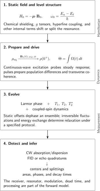
A magnetic-resonance spectrum or transient is the output of a complete Hamiltonian–preparation–evolution–detector chain. Relaxation parameters and instrument settings belong to the forward model, not merely to a correction applied after the spectrum is acquired.

Spin in a Static Magnetic Field

Magnetic coupling

A magnetic moment $\boldsymbol{\mu}$ in a magnetic flux density $\mathbf B$ has the interaction Hamiltonian

$$H_Z=-\boldsymbol{\mu}\cdot\mathbf B.$$

For an angular momentum $\mathbf J$ with gyromagnetic ratio $\gamma$,

$$\boldsymbol{\mu}=\gamma\mathbf J, \qquad H_Z=-\gamma\,\mathbf J\cdot\mathbf B.$$

The sign of $\gamma$ matters. It determines which magnetic projection lies lower in energy and the sense of precession. The positive transition frequency is instead defined by the energy gap,

$$\omega_0\equiv\frac{E_u-E_\ell}{\hbar}>0, \qquad \nu_0=\frac{\omega_0}{2\pi}.$$

For a spin-$1/2$ in $\mathbf B_0=B_0\hat{\mathbf z}$,

$$H_0=-\frac{\hbar\gamma B_0}{2}\sigma_z, \qquad \omega_0=|\gamma|B_0.$$

Keeping the signed $\gamma$ in the Hamiltonian while using a positive $\omega_0$ for the spectral gap avoids two common errors: reversing the energy ordering and assigning a negative measured frequency.

Magnetic resonance usually uses an effective Hamiltonian

The bare Zeeman term is only the first layer. The local field and spin couplings depend on electronic structure, neighboring spins, molecular orientation, and motion. A schematic NMR spin Hamiltonian is

$$\begin{aligned} \frac{H_{\mathrm{NMR}}}{\hbar} ={}& -\sum_k \gamma_k\, \mathbf B_0\cdot \bigl(\mathbf 1-\boldsymbol{\sigma}_k\bigr) \cdot\mathbf I_k \\ &+ 2\pi\sum_{k<\ell}J_{k\ell}\, \mathbf I_k\cdot\mathbf I_\ell \\ &+ \frac{H_{\mathrm{dip}}}{\hbar} + \frac{H_Q}{\hbar} \,+\cdots . \end{aligned}$$

Here the spin operators $\mathbf I_k$ are dimensionless, $\boldsymbol{\sigma}_k$ is a shielding tensor, $J_{k\ell}$ is an isotropic scalar coupling in hertz, $H_{\mathrm{dip}}$ contains direct magnetic dipole–dipole coupling, and $H_Q$ is a nuclear quadrupole interaction when $I\ge1$. Which terms survive or average out depends on phase, orientation, motion, and pulse sequence.

A common EPR effective Hamiltonian is

$$\begin{aligned} \frac{H_{\mathrm{EPR}}}{\hbar} ={}& \frac{\mu_B}{\hbar}\, \mathbf B_0\cdot\mathbf g\cdot\mathbf S + \mathbf S\cdot\mathbf A\cdot\mathbf I \\ &+ \mathbf S\cdot\mathbf D\cdot\mathbf S \,+\cdots , \end{aligned}$$

where $\mathbf S$ and $\mathbf I$ are dimensionless, and the tensors $\mathbf A$ and $\mathbf D$ are written in angular-frequency units. $\mathbf g$ describes the effective electron Zeeman interaction, $\mathbf A$ the electron–nuclear hyperfine coupling, and $\mathbf D$ a zero-field splitting, normally relevant for $S\ge1$.

These Hamiltonians are not universal templates into which every experiment must be forced. They are controlled low-energy models. Their parameters can depend on field, orientation, isotope, conformation, temperature, and the electronic states retained.

Transitions, not just levels

A transverse oscillating magnetic field couples through

$$V(t)=-\boldsymbol{\mu}\cdot\mathbf B_1(t).$$

The transition amplitude contains

$$\langle f| \boldsymbol{\mu}\cdot\boldsymbol{\epsilon}_1 |i\rangle,$$

where $\boldsymbol{\epsilon}_1$ is the drive polarization. For an unmixed angular-momentum multiplet and a transverse circular component, the familiar magnetic-dipole rule is $\Delta m=\pm1$. State mixing, anisotropic tensors, multiple coupled spins, forbidden-transition intensity borrowing, and orientation selection can all change the observed pattern.

The resonance condition

$$\hbar\omega_d=E_f(\mathbf B_0)-E_i(\mathbf B_0)$$

locates a possible transition. Its intensity additionally depends on the population difference, transition matrix element, saturation, relaxation, sample amount, resonator field, and detector response.

Larmor Frequency and Equilibrium Polarization

Precession

For the pure Zeeman Hamiltonian, the expectation value obeys

$$\frac{d\langle\mathbf J\rangle}{dt} = \gamma\, \langle\mathbf J\rangle\times\mathbf B_0.$$

The transverse component therefore rotates at the Larmor angular frequency. With

$$J_+\equiv J_x+iJ_y$$

and $\gamma B_0>0$,

$$\langle J_+(t)\rangle = \langle J_+(0)\rangle e^{-i\gamma B_0t}.$$

The sign in this complex representation depends on the definitions of $J_+$, $\gamma$, and the Fourier transform. The measurable spectral separation remains $\omega_0=|\gamma|B_0$ in the ideal spin-$1/2$ case.

An energy eigenstate has no transverse expectation value and therefore does not draw a classical-looking precession cone. A coherent superposition or an ensemble transverse magnetization does. This distinction is central to pulsed magnetic resonance.

Thermal population difference

For two levels separated by $\hbar\omega_0$ at temperature $T$, the equilibrium lower-minus-upper population difference is

$$p_\ell-p_u = \tanh\left( \frac{\hbar\omega_0}{2k_BT} \right).$$

In the high-temperature limit,

$$p_\ell-p_u \simeq \frac{\hbar\omega_0}{2k_BT}.$$

For room-temperature NMR this number is usually very small. A detectable signal comes from a macroscopic number of nuclei, resonant detection, signal averaging, and careful control of noise. The phrase “a $\pi$ pulse flips all spins” is therefore potentially misleading: the density operator is nearly maximally mixed, and the pulse rotates its small polarized deviation.

The equilibrium density operator is

$$\rho_{\mathrm{eq}} = \frac{e^{-\beta H_0}} {\operatorname{Tr}(e^{-\beta H_0})}, \qquad \beta=\frac{1}{k_BT}.$$

For a spin-$1/2$ with a suitably chosen lower-state direction,

$$\rho_{\mathrm{eq}} = \frac12 \left[ \mathbf 1 + \tanh\left( \frac{\beta\hbar\omega_0}{2} \right)\sigma_z \right].$$

If the basis or sign of $\gamma$ is reversed, the sign of the $\sigma_z$ term reverses as well. The Boltzmann weights, not a memorized sign, decide the physical population ordering.

Useful frequency scales

The 2022 CODATA recommended gyromagnetic ratios give approximately

$$\begin{aligned} \frac{\gamma_p}{2\pi} &= 42.57748\ \mathrm{MHz\,T^{-1}}, \\ \frac{|\gamma_e|}{2\pi} &= 28.02495\ \mathrm{GHz\,T^{-1}}. \end{aligned}$$

Thus a proton at $1\ \mathrm T$ resonates near $42.6\ \mathrm{MHz}$, while a nearly free electron at the same field resonates near $28.0\ \mathrm{GHz}$. Real EPR fields depend on the effective $g$ matrix; real NMR frequencies are shifted by shielding and coupling. These numbers set scales, not exact line assignments.

Resonant Driving

Laboratory and rotating frames

Take a static field along $z$ and write a linearly oscillating transverse field as

$$\mathbf B(t) = B_0\hat{\mathbf z} + 2B_1\cos(\omega_dt+\phi)\hat{\mathbf x}.$$

The factor of two makes $B_1$ the amplitude of either circular component. For an isolated spin-$1/2$, the co-rotating component then gives the on-resonance Rabi angular frequency

$$\Omega=|\gamma|B_1.$$

Authors who call the full linear-field amplitude $B_1$ instead obtain $\Omega=|\gamma|B_1/2$. Pulse calibrations are meaningless unless this amplitude convention is stated.

Under the rotating-wave approximation, a convenient rotating-frame Hamiltonian is

$$\begin{aligned} H_{\mathrm{rot}} ={}& \frac{\hbar}{2} \bigl[ -\Delta\sigma_z \\ &+ \Omega\cos\phi\,\sigma_x \\ &+ \Omega\sin\phi\,\sigma_y \bigr], \end{aligned}$$

with detuning

$$\Delta=\omega_d-\omega_0.$$

Changing the rotating-frame convention can reverse the displayed signs of $\Delta$ or $\phi$. Consistent predictions depend on

$$\Omega_{\mathrm{eff}} = \sqrt{\Omega^2+\Delta^2},$$

and on the direction of the effective rotating-frame field.

On exact resonance, a pulse has area

$$\Theta = \int_0^{t_p}\Omega(t)\,dt.$$

An ideal $\pi/2$ pulse creates maximum transverse coherence from a longitudinally polarized spin-$1/2$ ensemble; an ideal $\pi$ pulse inverts the Bloch-vector deviation. Finite bandwidth, field inhomogeneity, off-resonance rotation, coupling during the pulse, and relaxation make real pulses imperfect.

Resonance is a driven response

The exact matching condition $\Delta=0$ is not enough to predict a signal. For a closed two-level system initially in its lower state,

$$P_u(t) = \frac{\Omega^2}{\Omega_{\mathrm{eff}}^2} \sin^2\left( \frac{\Omega_{\mathrm{eff}}t}{2} \right).$$

This formula explains coherent Rabi oscillations, but most bulk magnetic-resonance signals are ensemble observables with relaxation, inhomogeneous offsets, coupled-spin evolution, and a receiver transfer function. The Rabi Oscillations First Encounter and Resonant Driving pages develop the isolated-system limit.

Frequency-swept and field-swept spectra

Two common acquisition modes are:

1. Frequency sweep: hold $\mathbf B_0$ fixed and vary $\omega_d$.
2. Field sweep: hold $\omega_d$ fixed and vary $B_0$ through the resonance condition.

If an isolated line has a locally linear frequency,

$$\omega_{if}(B) \simeq \omega_{if}(B_r) + \gamma_{\mathrm{eff}}(B-B_r),$$

then a small angular-frequency width maps to a field width as

$$\Delta B \simeq \frac{\Delta\omega} {|\gamma_{\mathrm{eff}}|}.$$

This conversion fails near avoided crossings, turning points, overlapping orientation patterns, and strongly nonlinear level shifts. A field-swept intensity also acquires the appropriate Jacobian and field-dependent instrument response. Field and frequency axes are not interchangeable labels.

Continuous-Wave Response

Continuous-wave (CW) magnetic resonance applies a weak or moderate near-monochromatic drive while monitoring a steady response. The detected quadratures can be phased into components that are conventionally called absorptive and dispersive.

For a single two-level ensemble described by phenomenological Bloch equations, the steady absorptive response has the schematic form

$$S_{\mathrm{abs}}(\Delta) \propto \frac{ \Omega T_2 M_0 }{ 1+(\Delta T_2)^2+\Omega^2T_1T_2 }.$$

In the weak-drive limit, division by the drive amplitude gives

$$\chi''(\Delta) \propto \frac{T_2} {1+(\Delta T_2)^2},$$

while the dispersive component is proportional, up to phase and sign conventions, to

$$\chi'(\Delta) \propto \frac{\Delta T_2^2} {1+(\Delta T_2)^2}.$$

The weak-drive absorption line is Lorentzian with angular-frequency half-width at half maximum

$$\Gamma_{\omega,\mathrm{HWHM}} = \frac{1}{T_2}.$$

Consequently,

$$\Delta\nu_{\mathrm{FWHM}} = \frac{1}{\pi T_2}$$

for this specific homogeneous exponential-dephasing model.

Saturation and power broadening

The dimensionless saturation parameter in the same model is

$$s=\Omega^2T_1T_2.$$

As $s$ approaches or exceeds unity, the population difference is depleted, the line broadens by the factor $\sqrt{1+s}$, and the signal no longer scales linearly with drive amplitude. The exact detected power dependence can also contain resonator loading, spatial variation of $B_1$, modulation amplitude, and receiver nonlinearity.

Therefore:

• a low-power linewidth may estimate $T_2$ only after inhomogeneous and instrumental broadening are controlled;
• a power-broadened linewidth is not an intrinsic $T_2$;
• line height is especially vulnerable to saturation and phase errors;
• integrated intensity is more robust than height in some regimes, but it is not automatically invariant under saturation or baseline processing.

In CW EPR, field modulation and lock-in detection commonly produce the derivative of the absorption line. The derivative extrema are not two separate resonances, and their peak-to-peak separation is not the absorption FWHM. The conversion depends on the line shape and on whether modulation broadening is negligible.

Pulsed Magnetic Resonance

Free-induction decay

A pulse can create a transverse magnetization

$$M_+(0)=M_x(0)+iM_y(0).$$

After the pulse, a simple ensemble free-induction decay (FID) is

$$M_+(t) = M_+(0) \exp\left( -\frac{t}{T_2^*} \right) e^{-i\omega_0t}.$$

The complex receiver records two quadratures. Fourier transformation maps the time-domain phase evolution to a frequency-domain spectrum. Receiver dead time, finite acquisition duration, sampling rate, digital filters, apodization, zero filling, and phase correction all affect the displayed spectrum.

$T_2^*$ is an observed ensemble dephasing time. It can include irreversible coherence loss and a distribution of approximately static resonance offsets. If the offset distribution is Gaussian, the FID envelope is generally Gaussian rather than the exponential written above. A single $T_2^*$ value is therefore a model-dependent summary of a decay shape.

Echoes

A Hahn echo applies a nominal $\pi/2$ pulse, allows free evolution for $\tau$, applies a $\pi$ pulse, and observes rephasing near $2\tau$:

$$\frac{\pi}{2} \;-\;\tau\;-\; \pi \;-\;\tau\;-\; \text{echo}.$$

For a spin with a static offset $\delta\omega$, the first interval adds phase $\delta\omega\tau$. The ideal $\pi$ pulse reverses the relative phase ordering, so the second interval cancels that static contribution at the echo. It does not reverse stochastic fluctuations, energy relaxation, diffusion through field gradients, exchange, pulse errors, or all many-spin interactions.

An echo envelope is often fitted as

$$S_{\mathrm{echo}}(2\tau) = S_0 \exp\left[ -\left( \frac{2\tau}{T_m} \right)^n \right],$$

where $T_m$ is an operational phase-memory time and $n$ describes the chosen stretched or compressed exponential model. In a simple homogeneous Markovian limit, $n=1$ and $T_m=T_2$. In real NMR and EPR experiments, the reported decay constant can depend on pulse spacing, sequence, spectral diffusion, instantaneous diffusion, molecular motion, and the subset of spins excited.

Fourier duality is not a complete interpretation

A decaying exponential and a Lorentzian are Fourier pairs, but the relation

$$\Delta\nu_{\mathrm{FWHM}}=\frac{1}{\pi T_2}$$

holds only when the same homogeneous exponential coherence controls both measurements. A static offset distribution can broaden a one-pulse spectrum while being substantially refocused by an echo. Conversely, a finite pulse, finite acquisition window, or receiver filter can set an apparent width without defining a microscopic relaxation time.

Nuclear Magnetic Resonance

NMR probes nuclei with nonzero spin. Radiofrequency fields drive transitions among nuclear-spin states, while the surrounding electrons and other nuclei encode chemical and structural information in the effective Hamiltonian.

Main spectral parameters

Chemical shielding. Induced electronic currents modify the field at a nucleus. In a simple isotropic liquid, the observed resonance can be written schematically as

$$\omega_k \simeq \gamma_kB_0(1-\sigma_k).$$

Because absolute shielding is difficult to measure directly, solution NMR usually reports a chemical shift relative to a reference. A common frequency-ratio convention is

$$\delta_k = 10^6 \frac{ \nu_k-\nu_{\mathrm{ref}} }{ \nu_{\mathrm{ref}} } \quad\text{ppm}.$$

Exact reference and reporting conventions are nucleus and community dependent. The sign, reference material, sample conditions, and operating frequency should be stated.

Scalar coupling. Through-bond electron-mediated couplings split resonances and correlate nuclei. For two spin-$1/2$ nuclei in the weakly coupled high-field limit,

$$\frac{H_J}{\hbar} = 2\pi J\,\mathbf I_1\cdot\mathbf I_2$$

reduces approximately to a secular $2\pi J I_{1z}I_{2z}$ term. Strong coupling, near-equivalent chemical shifts, and pulse evolution require the full coupled-spin Hamiltonian.

Dipolar and quadrupolar interactions. Direct dipole–dipole coupling is orientation dependent. Rapid isotropic molecular tumbling averages its first-order static contribution in ordinary liquid-state spectra, but its fluctuations drive relaxation and the interaction remains central in solids. Nuclei with $I\ge1$ also have electric quadrupole moments that couple to electric-field gradients and often relax rapidly.

What NMR can infer

Depending on the experiment, NMR can constrain:

• local chemical environments through chemical shifts;
• connectivity and conformation through scalar and dipolar couplings;
• molecular motion, exchange, and transport through line shapes and relaxation;
• distances and orientations through controlled multi-pulse experiments;
• populations and kinetics through resolved signals and exchange models.

None of these is read directly from one peak. Assignments combine a spin Hamiltonian, pulse-sequence response, reference convention, sample conditions, and often several complementary experiments.

Electron Paramagnetic Resonance

EPR probes systems with unpaired electron spin, including radicals, transition-metal ions, defects, triplet states, and spin-labeled molecules. IUPAC recommends electron paramagnetic resonance as the general term; electron spin resonance remains widely used.

Main spectral parameters

Effective g matrix. For an effective spin-$1/2$,

$$\frac{H_Z}{\hbar} = \frac{\mu_B}{\hbar} \mathbf B_0\cdot\mathbf g\cdot\mathbf S.$$

The resonance field depends on field orientation relative to $\mathbf g$. The phrase “$g$ tensor” is widespread, but IUPAC recommends g-matrix because the effective-spin coordinate basis can transform independently of the laboratory spatial basis. An isotropic free-electron-like estimate is

$$\hbar\omega_d \simeq g\mu_BB_r.$$

Departures from the free-electron $g$ value encode spin–orbit coupling and the electronic environment, but assigning them generally requires an appropriate electronic-structure and ligand-field model.

Hyperfine coupling. Electron–nuclear coupling

$$\frac{H_{\mathrm{hf}}}{\hbar} = \mathbf S\cdot\mathbf A\cdot\mathbf I$$

splits and mixes electron-spin transitions. Isotropic contact and anisotropic dipolar contributions respond differently to molecular motion and orientation.

Zero-field splitting. For many $S\ge1$ systems, electron–electron interactions and spin–orbit effects split the manifold even at zero applied field. A tensor form is

$$\frac{H_{\mathrm{ZFS}}}{\hbar} = \mathbf S\cdot\mathbf D\cdot\mathbf S.$$

The common $D$ and $E$ parameters are coordinate-dependent representations of a traceless tensor. They should not be treated as additional Zeeman frequencies independent of orientation and state mixing.

CW and pulsed EPR

Conventional CW EPR often holds the microwave frequency fixed and sweeps the magnetic field. Pulsed EPR applies microwave pulses and detects an FID or echo. The resonator bandwidth, microwave magnetic-field distribution, sample dielectric loss, pulse dead time, and phase cycling can determine which spins and pathways are visible.

EPR relaxation times are frequently much shorter than NMR times, but this is not a definition and has many exceptions. Electron spins can couple strongly to lattice motion, nearby nuclei, other electron spins, and conduction electrons. Temperature and field can change both $T_1$ and phase memory by orders of magnitude.

NMR and EPR Compared

Feature	NMR	EPR
Primary moment	Nuclear spin magnetic moment	Unpaired-electron magnetic moment
Typical drive	Radiofrequency	Microwave
Scale at $1\ \mathrm T$	Proton near $42.6\ \mathrm{MHz}$	Free-electron-like spin near $28.0\ \mathrm{GHz}$
Common spectral coordinates	Frequency or chemical shift	Magnetic field at fixed microwave frequency, or frequency
Central Hamiltonian parameters	Shielding, $J$ coupling, dipolar and quadrupolar terms	$\mathbf g$, hyperfine, zero-field splitting, exchange
Common time-domain signals	FID, spin echo, multidimensional coherences	Echo, FID, nutation, electron–nuclear correlation
Typical structural sensitivity	Chemical environment, connectivity, motion	Electronic structure, local symmetry, nearby nuclei, spin dynamics
Frequent experimental limitation	Low thermal polarization and spectral overlap	Short relaxation, resonator bandwidth, microwave dead time

These are tendencies, not boundaries. Nuclear and electron spins can be coupled and measured together; both fields use CW, pulsed, field-domain, and frequency-domain methods.

Relaxation: T₁, T₂, and T₂*

Relaxation times are operational parameters of a model and protocol. They are not immutable labels attached to a particle.

Longitudinal relaxation T₁

$T_1$ describes recovery of the longitudinal population difference toward its equilibrium value. In the simplest Bloch model,

$$\frac{dM_z}{dt} = -\frac{M_z-M_0}{T_1},$$

so

$$M_z(t) = M_0 + \bigl[M_z(0)-M_0\bigr]e^{-t/T_1}.$$

After ideal inversion, $M_z(0)=-M_0$ and

$$M_z(t) = M_0\left(1-2e^{-t/T_1}\right).$$

Inversion recovery, saturation recovery, and related sequences estimate $T_1$ with different sensitivity to pulse imperfections, exchange, and multi-exponential behavior. “Spin–lattice relaxation” emphasizes energy exchange with non-spin degrees of freedom, but the microscopic reservoir may be molecular motion, phonons, electrons, photons, or other modes.

Homogeneous transverse relaxation T₂

$T_2$ characterizes irreversible decay of transverse coherence in a stated model. In a simple rotating frame,

$$\frac{dM_+}{dt} = -\frac{M_+}{T_2} -i\Delta M_+,$$

with solution

$$M_+(t) = M_+(0)e^{-t/T_2}e^{-i\Delta t}.$$

An echo sequence is commonly used to suppress static offset inhomogeneity before fitting this decay. The result can still depend on pulse spacing and sequence because the noise spectrum is sampled through a sequence-dependent filter.

Inhomogeneous dephasing T₂*

$T_2^*$ summarizes the decay of ensemble transverse magnetization without refocusing. It can include:

• the irreversible processes contributing to $T_2$;
• static or slowly varying field inhomogeneity;
• distributions of shielding or $g$ values;
• unresolved couplings and orientation distributions;
• spatial gradients, susceptibility variations, and instrumental drift.

In a simple additive-rate Lorentzian model,

$$\frac{1}{T_2^*} \simeq \frac{1}{T_2} + \frac{1}{T_{\mathrm{inh}}}.$$

This rate sum is not general. A Gaussian offset distribution gives a Gaussian decay and combines widths differently. It is safer to report the fitted functional form and pulse protocol along with the time constant.

Relation among relaxation times

For a Markovian two-level system with upward and downward population rates $\Gamma_\uparrow$ and $\Gamma_\downarrow$, plus pure-dephasing rate $\Gamma_\phi$,

$$\frac{1}{T_1} = \Gamma_\uparrow+\Gamma_\downarrow,$$

and

$$\frac{1}{T_2} = \frac{\Gamma_\uparrow+\Gamma_\downarrow}{2} + \Gamma_\phi = \frac{1}{2T_1} + \frac{1}{T_\phi}.$$

Within this model,

$$T_2\le2T_1.$$

The inequality is not a universal theorem for every fitted decay in a multilevel, non-Markovian, exchanging, driven, or inhomogeneous system. Comparing a one-pulse $T_2^*$ with $2T_1$, for example, does not test the two-level homogeneous relation.

The canonical distinction between energy relaxation and phase loss is developed in Dephasing vs Dissipation.

Density Matrices and Bloch Equations

Bloch vector

Every spin-$1/2$ density operator can be written

$$\rho = \frac12 \left( \mathbf 1 +u\sigma_x +v\sigma_y +w\sigma_z \right),$$

or explicitly,

$$\rho = \frac12 \begin{pmatrix} 1+w & u-iv\\ u+iv & 1-w \end{pmatrix}.$$

The Bloch vector is

$$\mathbf r=(u,v,w), \qquad |\mathbf r|\le1.$$

For an ensemble of identical spin-$1/2$ moments, the measured magnetization is proportional to the corresponding spin expectation values:

$$\begin{aligned} M_x&=C\,u,\\ M_y&=C\,v,\\ M_z&=C\,w, \end{aligned}$$

where $C$ contains spin density, magnetic moment, filling factor, and normalization conventions. The complex transverse signal is proportional to

$$M_+=C(u+iv).$$

Thus the receiver is sensitive to off-diagonal density-matrix coherence in the energy basis. It does not perform a projective measurement of each spin and average the resulting classical arrows.

Phenomenological Bloch equations

The Bloch equations combine torque with separate longitudinal and transverse relaxation:

$$\begin{aligned} \frac{d\mathbf M}{dt} ={}& \gamma\,\mathbf M\times\mathbf B(t) \\ &- \frac{M_x}{T_2}\hat{\mathbf x} - \frac{M_y}{T_2}\hat{\mathbf y} \\ &- \frac{M_z-M_0}{T_1}\hat{\mathbf z}. \end{aligned}$$

They are remarkably effective for an isolated transition or a weakly interacting ensemble. They are phenomenological unless their rates and equilibrium state have been derived from a microscopic open-system model.

For a two-level Lindblad model, the density-matrix master equation leads to Bloch-vector equations with the rate relation given above. This connection clarifies:

• why transverse coherence decays under both population relaxation and pure dephasing;
• why a continuous resonant drive saturates the population difference;
• why positivity constrains independently chosen phenomenological rates;
• why thermal equilibrium requires both upward and downward transitions at finite temperature.

The full derivation and steady state live in Optical Bloch Equations. The word optical refers to a common application; the two-level mathematics also underlies magnetic resonance.

Where the two-level picture breaks

Real magnetic-resonance spectra often involve more than one isolated transition:

• a spin $I>1/2$ or $S>1/2$ has multiple magnetic sublevels;
• hyperfine, quadrupolar, and zero-field terms mix the Zeeman basis;
• coupled spins create product-state manifolds and multiple-quantum coherences;
• a broad pulse can excite several transitions simultaneously;
• orientation distributions produce powder patterns rather than single Lorentzians;
• exchange and motion can change the Hamiltonian during the experiment.

One can still propagate a density operator,

$$\rho(t) = \mathcal U(t)\rho(0)$$

for closed evolution, or a dynamical map for open evolution, but a single three-component Bloch vector no longer captures the state. Liouville-space and coupled-spin methods then replace the isolated-transition picture.

Detection and Instrument Response

NMR induction

A precessing transverse nuclear magnetization changes the magnetic flux through a receiver coil. Faraday induction gives

$$V(t)=-\frac{d\Phi(t)}{dt}.$$

The flux depends on coil geometry, sample filling factor, resonator response, and the spatial magnetization. Quadrature down-conversion converts the radiofrequency voltage into a complex baseband signal. Receiver phase then sets which displayed component appears absorptive or dispersive.

EPR microwave detection

An EPR resonator or transmission structure measures how the spin ensemble changes microwave absorption, reflection, or transmission. CW instruments often use field modulation and phase-sensitive detection. Pulsed instruments detect microwave FIDs or echoes after the high-power pulse has decayed sufficiently for the receiver to recover.

The recorded signal is therefore not simply $\langle S_x\rangle$. It is the spin response filtered by:

$$\begin{gathered} \text{resonator bandwidth and phase} \\ \quad+\quad\text{excitation profile} \\ +\quad \text{receiver dead time and gain} \\ +\quad \text{modulation or digitization} \\ +\quad \text{baseline and processing}. \end{gathered}$$

Calibration checklist

A defensible measurement records or calibrates:

1. static field magnitude, homogeneity, and sweep direction;
2. drive frequency, phase, power, pulse envelope, and $B_1$ calibration;
3. resonator frequency, bandwidth, loading, and sample placement;
4. receiver phase, gain, dead time, sampling rate, and filter settings;
5. temperature, sample concentration, isotope content, orientation, and preparation history;
6. modulation amplitude and frequency for derivative-detected CW spectra;
7. reference compound or field standard and the convention used;
8. processing steps, baseline model, apodization, and uncertainty.

A line center or relaxation time without this provenance may not be reproducible even when the numerical fit is precise.

A Forward Model for Interpretation

The most reliable reading strategy separates Hamiltonian parameters, dynamics, and detector effects.

Observable	Leading physical dependence	Important confounders
Resonance center	Energy difference and field/frequency calibration	Reference convention, field drift, Bloch–Siegert or other drive shifts
Splitting	Hyperfine, scalar, dipolar, quadrupolar, or zero-field coupling	Strong coupling, state mixing, overlap, orientation
Integrated intensity	Population difference and transition moment	Saturation, excitation bandwidth, relaxation, receiver transfer
Absorption linewidth	Homogeneous dephasing in the simplest limit	Inhomogeneity, power and modulation broadening, unresolved structure
FID decay	Offset distribution plus irreversible coherence loss	Dead time, radiation damping, windowing, diffusion
Echo decay	Unrefocused dynamics under a chosen sequence	Pulse errors, spectral diffusion, instantaneous diffusion, sequence filter
Receiver phase	Coherence phase and instrument reference	Cable delay, resonator phase, digital phase correction

Practical workflow

1. Write the smallest effective Hamiltonian justified by the sample and field regime.
2. Diagonalize it at the actual field and orientation; do not assume high-field quantum numbers before checking.
3. Compute transition frequencies and magnetic-dipole matrix elements.
4. Specify equilibrium or non-equilibrium populations.
5. Propagate the density operator under the actual CW or pulse sequence.
6. Add relaxation with a declared phenomenological or microscopic model.
7. Average over orientations, field distributions, conformers, isotopes, or exchange pathways as required.
8. Apply resonator, modulation, receiver, and processing response.
9. Fit all relevant data sets jointly when parameters are shared.
10. Report conventions, covariance, systematic uncertainty, and plausible alternative assignments.

This order prevents an attractive peak assignment from silently dictating the Hamiltonian used to “confirm” it.

Worked Examples

Proton and electron scales at the same field

At $B_0=3.00\ \mathrm T$, the ideal proton frequency is

$$\begin{aligned} \nu_p &= \left( 42.57748\ \mathrm{MHz\,T^{-1}} \right) \left( 3.00\ \mathrm T \right) \\ &= 127.732\ \mathrm{MHz}. \end{aligned}$$

The free-electron-like frequency is

$$\begin{aligned} \nu_e &= \left( 28.02495\ \mathrm{GHz\,T^{-1}} \right) \left( 3.00\ \mathrm T \right) \\ &= 84.0749\ \mathrm{GHz}. \end{aligned}$$

Their ratio is roughly $658$. This large scale separation explains the typical radiofrequency–microwave distinction, but chemical shielding and $g$-tensor anisotropy determine the fine structure.

A proton π/2 pulse

Suppose $B_1=0.100\ \mathrm{mT}$ is the co-rotating amplitude in the convention used above. Then

$$\begin{aligned} \frac{\Omega}{2\pi} &= \left( 42.57748\ \mathrm{MHz\,T^{-1}} \right) \\ &\quad\times \left( 1.00\times10^{-4}\ \mathrm T \right) \\ &= 4.25775\ \mathrm{kHz}. \end{aligned}$$

For a rectangular resonant $\pi/2$ pulse,

$$t_{\pi/2} = \frac{\pi/2}{\Omega} = \frac{1}{4(\Omega/2\pi)} \simeq 58.7\ \mu\mathrm s.$$

If $0.100\ \mathrm{mT}$ instead denoted the peak amplitude of the full linearly oscillating field, the co-rotating amplitude would be half as large and the pulse would take twice as long.

Linewidth and echo disagreement

Suppose a one-pulse spectrum has a Lorentzian-looking FWHM of $5.0\ \mathrm{kHz}$, while a Hahn-echo envelope gives $T_2=1.0\ \mathrm{ms}$. If the spectrum were homogeneously limited by this $T_2$, its expected FWHM would be

$$\Delta\nu_{\mathrm{hom}} = \frac{1}{\pi T_2} \simeq 318\ \mathrm{Hz}.$$

The measured line is much broader. Static field variation, a distribution of local shifts, unresolved couplings, or another inhomogeneous mechanism is therefore required. The discrepancy is evidence about the forward model, not a reason to choose whichever “$T_2$” looks more convenient.

Common Mistakes

Treating every spin as an isolated two-level system

Nuclear quadrupole, hyperfine, zero-field, and coupled-spin interactions can produce many levels and mixed eigenstates. Check the Hamiltonian before assigning $\Delta m=\pm1$ labels.

Dropping the sign of the gyromagnetic ratio everywhere

$|\gamma|B_0$ gives a positive ideal transition frequency, but the signed $\gamma$ determines energy ordering and precession direction.

Hiding the B₁ convention

A factor of two separates the peak amplitude of a linearly oscillating field from either circular component. State which amplitude defines $\Omega$.

Equating a spectral width with 1/T₂

Only a homogeneous exponential coherence produces the simple $\Delta\nu_{\mathrm{FWHM}}=1/(\pi T_2)$ relation. Inhomogeneity, unresolved structure, power, modulation, and the instrument can dominate.

Calling T₂* an intrinsic relaxation time

$T_2^*$ includes ensemble offset distributions and depends on the acquisition. Echoes can refocus some contributions.

Believing an echo reverses all decoherence

An ideal Hahn echo reverses static single-spin offsets. It does not reverse arbitrary noise, dissipation, diffusion, exchange, or many-body evolution.

Reading derivative EPR peaks as absorption peaks

Lock-in-detected CW EPR commonly displays a derivative. Its extrema and peak-to-peak width require a line-shape-specific conversion.

Assuming higher drive always gives better signal

Strong drive causes saturation, power broadening, off-resonant excitation, heating, and pulse artifacts. Signal-to-noise and interpretability can worsen.

Treating T₁ and T₂ as sample constants

They can depend on field, temperature, orientation, concentration, pulse spacing, transition, and fitted model. Report the protocol.

Ignoring the receiver

Phase, dead time, resonator bandwidth, modulation, and processing can move or suppress features. The instrument belongs in the forward model.

Key Takeaways

• Magnetic resonance measures driven transitions and coherences among magnetic states, not a bare magnetic moment in isolation.
• The static Zeeman term sets the scale; shielding, $g$ tensors, hyperfine, dipolar, scalar, quadrupolar, and zero-field terms create the information content.
• NMR and EPR share the same preparation–drive–evolution–detection logic while differing strongly in moments, frequencies, interactions, and instrumentation.
• CW spectra probe a driven steady state; pulsed methods prepare coherence and observe its time evolution.
• $T_1$ describes longitudinal recovery, $T_2$ homogeneous transverse coherence in a stated model, and $T_2^*$ unrefocused ensemble dephasing.
• The relation $1/T_2=1/(2T_1)+1/T_\phi$ belongs to a Markovian two-level model and should not be exported without checking its assumptions.
• A density matrix connects microscopic spin coherence to macroscopic magnetization, while the receiver and processing determine the recorded signal.

Exercises

Exercise 1: Field and frequency scales

Use

$$\begin{aligned} \frac{\gamma_p}{2\pi} &= 42.57748\ \mathrm{MHz\,T^{-1}}, \\ \frac{|\gamma_e|}{2\pi} &= 28.02495\ \mathrm{GHz\,T^{-1}}. \end{aligned}$$

1. Find the ideal proton and free-electron-like resonance frequencies at $B_0=7.00\ \mathrm T$.
2. Find the free-electron-like resonance field for $\nu_d=9.50\ \mathrm{GHz}$.
3. Explain why the last result is only an estimate for a real paramagnetic center.

Solution

For the proton,

$$\begin{aligned} \nu_p &= \left( 42.57748\ \mathrm{MHz\,T^{-1}} \right) \left( 7.00\ \mathrm T \right) \\ &= 298.042\ \mathrm{MHz}. \end{aligned}$$

For the electron,

$$\begin{aligned} \nu_e &= \left( 28.02495\ \mathrm{GHz\,T^{-1}} \right) \left( 7.00\ \mathrm T \right) \\ &= 196.175\ \mathrm{GHz}. \end{aligned}$$

At $9.50\ \mathrm{GHz}$,

$$B_r = \frac{ 9.50\ \mathrm{GHz} }{ 28.02495\ \mathrm{GHz\,T^{-1}} } \simeq 0.3390\ \mathrm T.$$

A real center has an effective $\mathbf g$ matrix, hyperfine coupling, and possibly zero-field or exchange terms. Its transition frequency can depend on orientation and state mixing, so $B_r$ must be computed from the complete effective Hamiltonian.

Exercise 2: Thermal proton polarization

Estimate the lower-minus-upper equilibrium population difference for protons at $B_0=14.1\ \mathrm T$ and $T=298\ \mathrm K$. Use the high-temperature approximation and

$$\begin{aligned} h &= 6.62607015\times10^{-34}\ \mathrm{J\,s}, \\ k_B &= 1.380649\times10^{-23}\ \mathrm{J\,K^{-1}}. \end{aligned}$$

What fraction of the spins contributes to the net two-level population imbalance?

Solution

The proton frequency is

$$\begin{aligned} \nu_p &= \left( 42.57748\ \mathrm{MHz\,T^{-1}} \right) \\ &\quad\times \left( 14.1\ \mathrm T \right) \\ &\simeq 600.34\ \mathrm{MHz}. \end{aligned}$$

Since $\hbar\omega_0=h\nu_p$,

$$\begin{aligned} p_\ell-p_u &\simeq \frac{h\nu_p}{2k_BT} \\ &= \frac{ 3.9780\times10^{-25}\ \mathrm J }{ 8.2287\times10^{-21}\ \mathrm J } \\ &\simeq 4.83\times10^{-5}. \end{aligned}$$

Only about $48$ parts per million form the net two-level population imbalance. Both levels remain almost equally populated. The macroscopic NMR signal is possible because the sample contains a very large number of nuclei.

Exercise 3: Pulse calibration and convention

A resonant proton pulse has a co-rotating amplitude $B_1=0.250\ \mathrm{mT}$.

1. Find $\Omega/2\pi$.
2. Find the rectangular $\pi/2$ and $\pi$ pulse durations.
3. How do the answers change if $0.250\ \mathrm{mT}$ was actually the peak amplitude of the full linearly oscillating field?

Solution

With the co-rotating convention,

$$\begin{aligned} \frac{\Omega}{2\pi} &= \left( 42.57748\ \mathrm{MHz\,T^{-1}} \right) \\ &\quad\times \left( 2.50\times10^{-4}\ \mathrm T \right) \\ &= 10.6444\ \mathrm{kHz}. \end{aligned}$$

Therefore

$$t_{\pi/2} = \frac{1}{4(\Omega/2\pi)} \simeq 23.49\ \mu\mathrm s,$$

and

$$t_\pi = \frac{1}{2(\Omega/2\pi)} \simeq 46.97\ \mu\mathrm s.$$

If the stated field is the peak linear amplitude, its co-rotating component is $0.125\ \mathrm{mT}$. The Rabi frequency is halved and both pulse durations double.

Exercise 4: Homogeneous linewidth and field conversion

An isolated EPR transition has $T_2=100\ \mathrm{ns}$ and is in the weak-drive homogeneous Lorentzian limit.

1. Find its absorption FWHM in hertz.
2. Convert this to a field FWHM using $|\gamma_e|/2\pi=28.02495\ \mathrm{GHz\,T^{-1}}$.
3. For a derivative of an ideal Lorentzian absorption line, show that the peak-to-peak derivative width is the absorption FWHM divided by $\sqrt3$.

Solution

The homogeneous frequency FWHM is

$$\begin{aligned} \Delta\nu_{\mathrm{FWHM}} &= \frac{1}{\pi T_2} \\ &= \frac{1}{\pi(100\times10^{-9}\ \mathrm s)} \\ &\simeq 3.183\ \mathrm{MHz}. \end{aligned}$$

In the locally linear field approximation,

$$\begin{aligned} \Delta B_{\mathrm{FWHM}} &= \frac{3.183} {28.02495\times10^3} \ \mathrm T \\ &\simeq 1.136\times10^{-4}\ \mathrm T \\ &= 0.1136\ \mathrm{mT}. \end{aligned}$$

Write the absorption Lorentzian as

$$L(x)=\frac{1}{1+(x/\Gamma)^2},$$

where $\Gamma$ is the HWHM. Its derivative extrema satisfy

$$\frac{d^2L}{dx^2}=0,$$

which gives

$$x=\pm\frac{\Gamma}{\sqrt3}.$$

The derivative peak-to-peak separation is therefore

$$\Delta x_{\mathrm{pp}} = \frac{2\Gamma}{\sqrt3} = \frac{ \Delta x_{\mathrm{FWHM}} }{\sqrt3}.$$

This result assumes negligible modulation broadening and a true Lorentzian absorption line.

Exercise 5: Extracting a pure-dephasing time

A two-level transition is well described by a Markovian relaxation model. Measurements give

$$T_1=1.20\ \mathrm s, \qquad T_2=80.0\ \mathrm{ms}.$$

Find $T_\phi$. Check the $T_2\le2T_1$ consistency condition. Would the same calculation be justified if the $80.0\ \mathrm{ms}$ value were a one-pulse $T_2^*$?

Solution

Use

$$\frac{1}{T_\phi} = \frac{1}{T_2} - \frac{1}{2T_1}.$$

Numerically,

$$\begin{aligned} \frac{1}{T_\phi} &= \frac{1}{0.0800\ \mathrm s} - \frac{1}{2(1.20\ \mathrm s)} \\ &= 12.500\ \mathrm{s^{-1}} - 0.4167\ \mathrm{s^{-1}} \\ &= 12.083\ \mathrm{s^{-1}}. \end{aligned}$$

Thus

$$T_\phi\simeq82.8\ \mathrm{ms}.$$

The inequality is easily satisfied because

$$80.0\ \mathrm{ms}<2.40\ \mathrm s.$$

A one-pulse $T_2^*$ may contain static inhomogeneity, so inserting it into the homogeneous Markovian rate relation would incorrectly attribute reversible ensemble dephasing to microscopic pure dephasing.

Exercise 6: What a Hahn echo refocuses

An ensemble has static angular-frequency offsets $\delta\omega_j$ around the carrier. Ignore all interactions during ideal instantaneous pulses.

1. Show that the transverse phase acquired before and after an ideal $\pi$ pulse cancels at time $2\tau$.
2. Add homogeneous decay with time $T_2$ and find the echo amplitude.
3. Explain why a fluctuating offset need not cancel.

Solution

During the first interval, spin $j$ acquires the relative phase

$$\phi_j^{(1)}=\delta\omega_j\tau.$$

The $\pi$ pulse reverses the transverse phase ordering. During the second interval the same static offset contributes

$$\phi_j^{(2)}=-\delta\omega_j\tau.$$

Hence

$$\phi_j(2\tau) = \phi_j^{(1)}+\phi_j^{(2)} = 0$$

for every static offset, so the ensemble rephases.

Homogeneous exponential coherence loss continues through both intervals:

$$S_{\mathrm{echo}}(2\tau) = S_0e^{-2\tau/T_2}.$$

If the offset changes in time, the accumulated phase is an integral over the noise before and after the pulse. The two integrals cancel only for noise components that are sufficiently static or symmetric under the sequence. Rapid fluctuations, energy relaxation, and many-spin evolution generally remain.

Exercise 7: Density matrix and quadrature signal

Consider

$$\rho = \frac12 \begin{pmatrix} 1.3 & 0.6+0.2i\\ 0.6-0.2i & 0.7 \end{pmatrix}.$$

1. Identify $(u,v,w)$ in $\rho=(\mathbf1+u\sigma_x+v\sigma_y+w\sigma_z)/2$.
2. Check positivity.
3. Find the normalized complex transverse signal $M_+/C=u+iv$.
4. What happens to its magnitude during ideal static-field precession?

Solution

Comparison with

$$\rho = \frac12 \begin{pmatrix} 1+w & u-iv\\ u+iv & 1-w \end{pmatrix}$$

gives

$$u=0.6, \qquad v=-0.2, \qquad w=0.3.$$

The Bloch-vector length is

$$\begin{aligned} |\mathbf r| &= \sqrt{0.36+0.04+0.09} \\ &= 0.7\le1, \end{aligned}$$

so the density operator is positive. Its eigenvalues are

$$\lambda_\pm = \frac{1\pm|\mathbf r|}{2} = 0.85,\ 0.15.$$

The normalized complex transverse signal is

$$\frac{M_+}{C} = 0.6-0.2i,$$

with magnitude

$$\begin{aligned} \frac{|M_+|}{C} &= \sqrt{0.36+0.04} \\ &= \sqrt{0.40} \\ &\simeq 0.632. \end{aligned}$$

Ideal static-field precession changes only its complex phase:

$$M_+(t)=M_+(0)e^{-i\omega_0t}.$$

Its magnitude stays fixed until relaxation or ensemble dephasing is added.

Exercise 8: Diagnose a power-dependent CW line

A field-swept CW EPR line broadens and decreases in peak derivative amplitude as microwave power is raised. Its center remains fixed. At the same temperature, a low-power echo experiment gives a phase-memory time that would predict a narrower homogeneous absorption line than the lowest-power CW spectrum.

Construct a sequence of tests that distinguishes saturation and power broadening from static inhomogeneity, unresolved hyperfine structure, modulation broadening, and instrumental distortion.

Solution

A defensible diagnosis separates one mechanism at a time:

1. Measure peak height, integrated absorption, and linewidth over a broad low-power range. Verify the expected linear-response power scaling before fitting a saturation model.
2. Independently measure or estimate $T_1$ and the relevant echo decay, then compare the onset of broadening with $s=\Omega^2T_1T_2\sim1$ using a calibrated $B_1$.
3. Reduce the field-modulation amplitude and extrapolate the linewidth toward zero modulation.
4. Change resonator loading, sample amount, and receiver gain to test cavity and detection nonlinearity.
5. Acquire spectra at several microwave frequencies or sample orientations. A $g$ distribution, powder pattern, or unresolved hyperfine structure transforms differently from a homogeneous width.
6. Compare absorption reconstructed from the derivative with a direct or independently phased measurement, including baseline uncertainty.
7. Vary pulse bandwidth and field position in the echo experiment to test whether it selects only a narrow subset of the CW ensemble.
8. Repeat over temperature. Saturation follows both $T_1$ and $T_2$, while static disorder and unresolved structure may show different trends.

The power dependence supports saturation, but the excess low-power CW width shows that saturation is not the only mechanism. A joint forward model should include homogeneous response, static distributions or unresolved transitions, modulation, and resonator response.

Further Connections

• Spectroscopy Overview supplies the general preparation–interaction–evolution–detection framework.
• Transition Rates develops the population and matrix-element factors behind weak absorption.
• Line Shapes and Broadening distinguishes homogeneous, inhomogeneous, instrumental, and finite-time widths.
• Selection Rules in Spectroscopy explains exact rules, approximate propensities, and intensity borrowing.
• Zeeman Effect in Atoms and Hyperfine Structure own atomic magnetic sublevel structure.
• Magnetic Moments and g Factors defines gyromagnetic ratios and effective $g$ factors.
• Rotating-Wave Approximation derives the co-rotating effective Hamiltonian and its validity conditions.
• Bloch Sphere gives the geometry and positivity of spin-$1/2$ density operators.
• Rabi and Ramsey Control develops separated-field phase accumulation and precision readout.
• Magnetometry develops field measurands, atomic-vapor architectures, SERF operation, sensitivity spectra, calibration, and heading systematics.

References

• IUPAC, “nuclear magnetic resonance spectroscopy,” Compendium of Chemical Terminology, 5th ed. — operational NMR definition and terminology.
• IUPAC, “electron paramagnetic resonance,” Compendium of Chemical Terminology, 5th ed. — recommended EPR terminology and definition.
• IUPAC, “relaxation time,” Compendium of Chemical Terminology, 5th ed. — longitudinal and transverse magnetic-resonance usage.
• R. K. Harris et al., “NMR Nomenclature: Nuclear Spin Properties and Conventions for Chemical Shifts,” Pure and Applied Chemistry 73, 1795–1818 (2001), doi:10.1351/pac200173111795 — nucleus, frequency, and chemical-shift conventions.
• R. K. Harris et al., “Further Conventions for NMR Shielding and Chemical Shifts,” Pure and Applied Chemistry 80, 59–84 (2008), doi:10.1351/pac200880010059 — reference and shielding recommendations.
• H. Kon, “Recommendations for EPR/ESR Nomenclature and Conventions for Presenting Experimental Data in Publications (Recommendations 1989),” Pure and Applied Chemistry 61, 2195–2200 (1989), doi:10.1351/pac198961122195 — EPR quantities, units, and conventions.
• E. Tiesinga, P. J. Mohr, D. B. Newell, and B. N. Taylor, “CODATA Recommended Values of the Fundamental Physical Constants: 2022,” Journal of Physical and Chemical Reference Data 54, 033105 (2025), doi:10.1063/5.0279860 — proton and electron gyromagnetic-ratio values used for scale estimates.
• I. I. Rabi, S. Millman, P. Kusch, and J. R. Zacharias, “The Molecular Beam Resonance Method for Measuring Nuclear Magnetic Moments,” Physical Review 55, 526–535 (1939), doi:10.1103/PhysRev.55.526 — resonant-transition method in molecular beams.
• F. Bloch, “Nuclear Induction,” Physical Review 70, 460–474 (1946), doi:10.1103/PhysRev.70.460 — nuclear induction, phenomenological dynamics, and finite relaxation times.
• E. M. Purcell, H. C. Torrey, and R. V. Pound, “Resonance Absorption by Nuclear Magnetic Moments in a Solid,” Physical Review 69, 37–38 (1946), doi:10.1103/PhysRev.69.37 — bulk nuclear resonance absorption.
• N. Bloembergen, E. M. Purcell, and R. V. Pound, “Relaxation Effects in Nuclear Magnetic Resonance Absorption,” Physical Review 73, 679–712 (1948), doi:10.1103/PhysRev.73.679 — microscopic motion and nuclear magnetic relaxation.
• E. L. Hahn, “Spin Echoes,” Physical Review 80, 580–594 (1950), doi:10.1103/PhysRev.80.580 — spin echoes and refocusing of reversible dephasing.
• F. Bloch and A. Siegert, “Magnetic Resonance for Nonrotating Fields,” Physical Review 57, 522–527 (1940), doi:10.1103/PhysRev.57.522 — counter-rotating-field resonance shift.
• A. Abragam, The Principles of Nuclear Magnetism, Oxford University Press, 1961 — spin Hamiltonians, line shapes, relaxation, and resonance methods.
• C. P. Slichter, Principles of Magnetic Resonance, 3rd ed., Springer, 1990, doi:10.1007/978-3-662-09441-9 — authoritative treatment of NMR dynamics and condensed-matter applications.
• R. R. Ernst, G. Bodenhausen, and A. Wokaun, Principles of Nuclear Magnetic Resonance in One and Two Dimensions, Oxford University Press, 1987 — density operators, pulses, coherence transfer, and multidimensional NMR.
• M. H. Levitt, Spin Dynamics: Basics of Nuclear Magnetic Resonance, 2nd ed., Wiley, 2008, doi:10.1002/9780470517123 — modern spin-dynamical and density-operator treatment.
• A. Schweiger and G. Jeschke, Principles of Pulse Electron Paramagnetic Resonance, Oxford University Press, 2001 — EPR effective Hamiltonians, pulse excitation, echoes, and electron–nuclear methods.
• J. A. Weil and J. R. Bolton, Electron Paramagnetic Resonance: Elementary Theory and Practical Applications, 2nd ed., Wiley, 2007, doi:10.1002/9780470084984 — CW EPR spectra, tensors, hyperfine structure, and instrumentation.