Zeeman Effect in Atoms

The Zeeman effect in atoms is the field-dependent shifting, splitting, and mixing of atomic energy levels produced by an applied magnetic field. A spectrum displays differences between those shifted levels, so its component frequencies, strengths, and polarizations depend on both the upper and lower states.

There is no field scale that is simply “weak” or “strong.” The useful quantum numbers change as the magnetic energy is compared successively with hyperfine, fine-structure, and electronic separations. A field can destroy $F$ as a good label while leaving $J$ almost exact, and a much larger field can decouple $L$ and $S$ without yet reorganizing the orbital motion.

This page owns that atom-specific regime map, the ground-state Breit–Rabi crossover, polarization-resolved line patterns, and experimental interpretation. Zeeman Effect as a Perturbation Example owns the generic minimal-coupling expansion, degenerate perturbation workflow, and a solvable spin–orbit crossover. Magnetic Moments and g-Factors owns sign conventions in their general setting, while Zeeman Effect Revisited owns the historical normal-versus-anomalous story. Magnetometry owns the instrument-level field measurand, optical pumping and readout, response, calibration, and systematic effects.

Normal and Anomalous Zeeman Patterns

The historical distinction concerns spectral patterns, not two different fundamental interactions.

In the normal Zeeman effect, electron spin does not contribute to the term magnetic moment, as for a pure singlet term with $S=0$. Then $J=L$ and $g_J\simeq1$. For an electric-dipole transition between two such levels, the frequency shift is

$$\begin{aligned} h\,\delta\nu &=\mu_BB \left(m_u-m_l\right) \\ &=q\mu_BB, \qquad q=0,\pm1. \end{aligned}$$

Only three frequency displacements occur: an unshifted $\pi$ component and two symmetrically shifted $\sigma$ components. Each component can still contain several transitions that coincide in frequency.

The anomalous Zeeman effect is the generic weak-field pattern when spin and orbital angular momentum are coupled. If the upper and lower levels have different Landé factors,

$$h\,\delta\nu_{ul} = \mu_BB \left(g_um_u-g_lm_l\right),$$

the allowed pairs of magnetic substates need not collapse to three frequencies. “Anomalous” is therefore historical language inherited from the spinless model. Modern angular-momentum theory predicts these patterns without anomaly.

For a nearly pure alkali doublet with $g_L\simeq1$ and $g_S\simeq2$, the leading electronic factors are

Level	$L$	$S$	$J$	Approximate $g_J$
${}^{2}S_{1/2}$	$0$	$1/2$	$1/2$	$2$
${}^{2}P_{1/2}$	$1$	$1/2$	$1/2$	$2/3$
${}^{2}P_{3/2}$	$1$	$1/2$	$3/2$	$4/3$

The alkali D lines consequently show anomalous electronic patterns even before nuclear spin is resolved. Hyperfine structure then adds $F,m_F$ sublevels and a still finer field scale.

Magnetic Moments and the Atomic Hamiltonian

Take the static field to define the quantization axis,

$$\mathbf B=B\hat{\mathbf z}, \qquad B\geq0.$$

For an atom described by electronic orbital angular momentum $\mathbf L$, electronic spin $\mathbf S$, and nuclear spin $\mathbf I$, the leading linear interaction may be written

$$H_Z = \frac{\mu_BB}{\hbar} \left( g_LL_z+g_SS_z+g_I'I_z \right).$$

Here $g_L$ and $g_S$ use the conventional positive coefficients in the energy Hamiltonian. The negative electronic charge is already included: the electron magnetic moment points oppositely to its angular momentum, so $-\boldsymbol\mu_e\cdot\mathbf B$ gives the positive electronic terms above.

For the nucleus, define its physical moment and a Bohr-magneton-scale coefficient by

$$\boldsymbol\mu_I = g_I\mu_N\frac{\mathbf I}{\hbar}, \qquad g_I' = -g_I\frac{\mu_N}{\mu_B}.$$

Then the nuclear Zeeman energy is $g_I'\mu_BBI_z/\hbar$. This prime convention prevents a common factor-of-$m_p/m_e$ mistake: $g_I$ is naturally paired with the nuclear magneton $\mu_N$, whereas $g_I'$ is the much smaller coefficient used beside electronic terms measured in $\mu_B$.

At 2022 CODATA precision,

$$\begin{aligned} \frac{\mu_B}{h} &\simeq 13.9962\ \mathrm{GHz\,T^{-1}}, \\ &\simeq 1.39962\ \mathrm{MHz\,G^{-1}}. \end{aligned}$$

This conversion is useful for estimates, but the relevant small parameter is a magnetic matrix element divided by a particular zero-field separation.

The linear Hamiltonian is not always complete. Minimal coupling also produces an explicit diamagnetic term proportional to $B^2$, and the linear interaction produces second-order shifts through virtual mixing. At still larger fields, neighboring electronic terms and orbital wavefunctions reorganize. Those effects set the boundary of a simple Zeeman model rather than a new universal Zeeman formula.

Landé Factors

Suppose spin–orbit coupling has already formed a level of fixed $L,S,J$. Projecting $\mathbf L$ and $\mathbf S$ onto $\mathbf J$ gives

$$\begin{aligned} g_J&=g_LC_L+g_SC_S, \\ C_L&= \frac{ J(J+1)+L(L+1)-S(S+1) }{2J(J+1)}, \\ C_S&= \frac{ J(J+1)-L(L+1)+S(S+1) }{2J(J+1)}. \end{aligned}$$

With $g_L=1$ and $g_S=2$, this reduces to the familiar Landé expression

$$g_J = 1+ \frac12 \left[ 1+ \frac{S(S+1)-L(L+1)}{J(J+1)} \right].$$

The formula assumes a sufficiently pure $LS$-coupled level and $J\ne0$. Configuration interaction, relativistic corrections, recoil, and the electron anomalous magnetic moment shift measured factors away from the simple rational values. A $J=0$ level has no first-order vector Zeeman shift within its one-dimensional manifold, but it can have a quadratic shift from mixing with other levels.

If hyperfine coupling next forms $\mathbf F=\mathbf I+\mathbf J$, the corresponding weak-field factor is

$$\begin{aligned} g_F&=g_JC_J+g_I'C_I, \\ C_J&= \frac{ F(F+1)+J(J+1)-I(I+1) }{2F(F+1)}, \\ C_I&= \frac{ F(F+1)+I(I+1)-J(J+1) }{2F(F+1)}. \end{aligned}$$

The nuclear term is small but should not be discarded in precision work. For $F=0$, the displayed ratio is not used; rotational symmetry gives no linear vector shift, while second-order mixing can remain.

These are projected coefficients, not immutable properties of a branch at every field. Once the field appreciably mixes different $F$ or $J$ manifolds, the slope $dE/dB$ evolves with the eigenvector.

Weak-Field Zeeman Effect

The word weak must name the coupling that remains dominant.

Fine structure resolved, hyperfine structure ignored

If

$$g_J\mu_BB \ll \Delta E_{\mathrm{fs}},$$

then $J,m_J$ are useful labels within an isolated fine-structure level. To first order,

$$E_{Jm_J}(B) = E_J(0) +g_J\mu_Bm_JB.$$

The $2J+1$ sublevels form an equally spaced fan only within that fixed level. A transition between two fans generally has unequal and nonuniformly repeated component frequencies because $g_u$ and $g_l$ differ.

Hyperfine structure resolved

If the still stronger condition

$$g_J\mu_BB \ll \Delta E_{\mathrm{hfs}}$$

holds, $F,m_F$ remain useful and

$$\begin{aligned} E_{Fm_F}(B) ={}& E_F(0)+g_F\mu_Bm_FB \\ &+O(B^2). \end{aligned}$$

The first-order slope is opposite for hyperfine manifolds whose $g_F$ factors have opposite signs. A state with $m_F=0$ has no linear shift in this approximation, but “no linear shift” does not mean field independent.

What remains exact

At fixed $B\hat{\mathbf z}$, full rotational symmetry is reduced to rotations about $z$. The projection along the field remains conserved in the ideal axial Hamiltonian even when the magnitude label changes:

$$m_F=m_I+m_J=m_I+m_L+m_S.$$

Parity also survives a uniform magnetic field for a parity-invariant atom because $\mathbf B$ is an axial vector. Thus intermediate-field calculations should be block diagonalized by exact labels such as projection and parity, not by a zero-field label that the field has already mixed.

Hierarchy	Useful labels	Leading treatment
magnetic energy below hyperfine splitting	$F,m_F$	use $g_Fm_F$
magnetic energy comparable to hyperfine splitting	$m_F$ exact; $F$ mixed	diagonalize fixed-$m_F$ blocks
above hyperfine but below fine structure	$m_I,m_J$	treat hyperfine coupling as smaller
comparable to fine structure	total projection exact; $J$ mixed	diagonalize spin–orbit and Zeeman terms together
above fine structure but below electronic gaps	$m_I,m_L,m_S$	treat spin–orbit coupling as smaller

The Two Paschen–Back Crossovers

The phrase Paschen–Back regime is incomplete until it names the angular momenta that decouple.

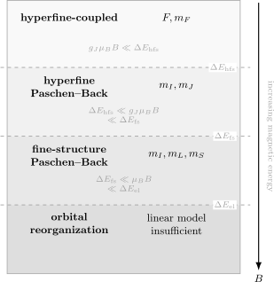
An atomic field scan can cross two distinct coupling scales. Hyperfine Paschen–Back behavior decouples $\mathbf I$ from $\mathbf J$; fine-structure Paschen–Back behavior decouples $\mathbf L$ from $\mathbf S$. Beyond electronic gaps or appreciable diamagnetic energy, the linear Zeeman model itself is no longer sufficient.

Hyperfine Paschen–Back regime

When

$$\Delta E_{\mathrm{hfs}} \ll g_J\mu_BB \ll \Delta E_{\mathrm{fs}},$$

$J$ remains well defined but $F$ does not. The useful basis approaches $\lvert Jm_J\rangle\lvert Im_I\rangle$. For a magnetic-dipole hyperfine Hamiltonian,

$$H_{\mathrm{hfs}} = \frac{A}{\hbar^2} \mathbf I\cdot\mathbf J,$$

the leading strong-field energy is

$$\begin{aligned} E(m_J,m_I) \simeq{}& g_J\mu_Bm_JB +g_I'\mu_Bm_IB \\ &+A m_Im_J. \end{aligned}$$

Off-diagonal hyperfine terms give corrections suppressed by the magnetic separation. Electric-quadrupole hyperfine structure and nearby fine-structure levels must be retained when their target accuracy requires them.

Fine-structure Paschen–Back regime

At a much larger field,

$$\Delta E_{\mathrm{fs}} \ll \mu_BB \ll \Delta E_{\mathrm{el}},$$

$L$ and $S$ decouple relative to the field. The basis approaches $\lvert Lm_L\rangle\lvert Sm_S\rangle$, with leading electronic energy

$$E_Z \simeq \mu_BB \left(g_Lm_L+g_Sm_S\right).$$

Spin–orbit coupling then supplies a smaller correction and can still mix uncoupled states with the same total projection. The right-hand inequality matters: if the field also competes with electronic term separations or the explicit diamagnetic energy, the orbitals themselves must be recalculated.

States evolve continuously through both crossovers. The labels change because a different part of the Hamiltonian becomes nearly diagonal, not because a quantum number jumps discontinuously inside an eigenvector.

Breit–Rabi Ground-State Crossover

An alkali ground state has $L=0$ and $J=1/2$. If its hyperfine structure is dominated by the magnetic-dipole constant $A$, the Hamiltonian

$$H = \frac{A}{\hbar^2} \mathbf I\cdot\mathbf J + \frac{\mu_BB}{\hbar} \left(g_JJ_z+g_I'I_z\right)$$

can be diagonalized analytically.

The exact projection

$$m=m_F=m_I+m_J$$

defines independent blocks. For a nonstretched value of $m$, choose

$$\begin{aligned} \lvert +\rangle &= \left\lvert m_J=\frac12, m_I=m-\frac12 \right\rangle, \\ \lvert -\rangle &= \left\lvert m_J=-\frac12, m_I=m+\frac12 \right\rangle. \end{aligned}$$

In this basis,

$$\begin{aligned} H_m ={}& -\frac{A}{4} +g_I'\mu_BmB \\ &+ \frac12 \begin{pmatrix} D_m & C_m \\ C_m & -D_m \end{pmatrix}, \end{aligned}$$

where

$$\begin{aligned} D_m &=Am+ \left(g_J-g_I'\right)\mu_BB, \\ C_m &=A \sqrt{ \left(I+\frac12\right)^2-m^2 }. \end{aligned}$$

The off-diagonal element is the spin-exchange part of $\mathbf I\cdot\mathbf J$. It vanishes for stretched projections because only one uncoupled basis state exists there.

Define the zero-field hyperfine interval and dimensionless field by

$$\Delta E_{\mathrm{hfs}} = A\left(I+\frac12\right),$$ $$x = \frac{ \left(g_J-g_I'\right)\mu_BB }{\Delta E_{\mathrm{hfs}}}.$$

The two eigenvalues are the Breit–Rabi formula,

$$\begin{aligned} E_{\pm,m}(B) ={}& -\frac{\Delta E_{\mathrm{hfs}}}{2(2I+1)} +g_I'\mu_BmB \\ &\pm \frac{\Delta E_{\mathrm{hfs}}}{2} R_m(x), \\ R_m(x) ={}& \sqrt{ 1+ \frac{4m}{2I+1}x +x^2 }. \end{aligned}$$

For $A>0$, the plus and minus branches correlate at $B=0$ with $F=I+1/2$ and $F=I-1/2$, respectively. At $|x|\gg1$, their eigenvectors approach uncoupled $m_J,m_I$ states. Levels with the same $m$ repel because $C_m\ne0$; levels in different exact-$m$ sectors may cross.

The stretched states $m=\pm(I+1/2)$ are one dimensional. Their energies are obtained directly:

$$E_{\mathrm{str}}^{(\pm)} = \frac{AI}{2} \pm \mu_BB \left( \frac{g_J}{2}+g_I'I \right).$$

Using the square-root formula for a stretched branch without tracking which sign survives is a frequent source of spurious states.

Quadratic clock shift

For integer $m=0$, the transition between the two hyperfine branches has

$$\nu_{00}(B) = \nu_{\mathrm{hfs}} \sqrt{1+x^2},$$

where $\Delta E_{\mathrm{hfs}}=h\nu_{\mathrm{hfs}}$. Its small-field expansion is

$$\begin{aligned} \delta\nu_{00} &= \nu_{00}(B)-\nu_{\mathrm{hfs}} \\ &\simeq \frac{ \left(g_J-g_I'\right)^2 }{2\nu_{\mathrm{hfs}}} \left(\frac{\mu_BB}{h}\right)^2. \end{aligned}$$

Thus the $m_F=0$ clock transition is first-order insensitive near zero field but has a positive quadratic Zeeman shift in this ideal model.

Rubidium-87 example

For the $5{}^2S_{1/2}$ ground state of $^{87}\mathrm{Rb}$,

$$\begin{aligned} I&=\frac32, \\ \frac{\Delta E_{\mathrm{hfs}}}{h} &= 6.834682610904290(90)\ \mathrm{GHz}. \end{aligned}$$

Evaluated alkali data give approximately

$$\begin{aligned} g_J&=2.002331070, \\ g_I'&=-0.0009951414. \end{aligned}$$

The scale $x=1$ is therefore

$$B_0 = \frac{\Delta E_{\mathrm{hfs}}} {(g_J-g_I')\mu_B} \simeq 0.2438\ \mathrm T.$$

This is about $2438\ \mathrm G$: a field can be large on the ground-state hyperfine scale while remaining small compared with the alkali fine-structure splitting. The same constants give the weak-field clock coefficient

$$\frac{\delta\nu_{00}}{B^2} \simeq 575.15\ \mathrm{Hz\,G^{-2}}.$$

Excited-state hyperfine intervals are often much smaller, so their hyperfine Paschen–Back crossover can occur at substantially lower fields than the ground-state crossover. A single phrase such as “rubidium is in a strong field” is therefore insufficient; upper and lower levels must be classified separately.

Selection Rules and Polarization

In a weak-field hyperfine basis, an electric-dipole matrix element factorizes as

$$\begin{aligned} \mathcal M_q \propto{}& (-1)^{F_u-m_u} \begin{pmatrix} F_u & 1 & F_l \\ -m_u & q & m_l \end{pmatrix} \\ &\times \left\langle \alpha_uF_u \middle\|d\middle\| \alpha_lF_l \right\rangle. \end{aligned}$$

The $3j$ symbol enforces

$$m_u=m_l+q, \qquad q=0,\pm1.$$

The spherical polarization and magnetic selection rule are linked:

Component	Spherical index	Weak-field rule	Observation along $\mathbf B$	Observation perpendicular to $\mathbf B$
$\pi$	$q=0$	$\Delta m=0$	absent for ideal dipole radiation	linear, electric field parallel to $\mathbf B$
$\sigma^+$	$q=+1$	$\Delta m=+1$	circular	linear, electric field perpendicular to $\mathbf B$
$\sigma^-$	$q=-1$	$\Delta m=-1$	opposite circular sense	linear, electric field perpendicular to $\mathbf B$

The handedness assigned to $\sigma^+$ and $\sigma^-$ must state the propagation or viewing direction. Reversing that direction reverses the apparent circular handedness even though the atomic rule $q=\pm1$ is unchanged.

The symbol $m$ changes meaning with regime. It is $m_F$ when hyperfine coupling is good, $m_J$ after hyperfine decoupling, and $m_L$ for the leading electric-dipole orbital rule in the fine-structure Paschen–Back limit. Because the electric dipole operator acts on electronic coordinates, $\Delta m_I=0$ is the leading uncoupled-basis rule. Field-induced mixing spreads strength among components and can make nominally forbidden lines weakly allowed.

Frequencies alone do not determine a pattern. Relative intensity contains the squared angular coefficient, the reduced matrix element, the initial-state population, the driving polarization, and the observation geometry. Repeated absorption and spontaneous emission can optically pump population into stretched or dark states, so a strong line in an unpolarized thermal ensemble may become weak in a driven steady state.

Experimental Interpretation

Levels are not lines

For every observed component, form the difference

$$h\nu_{ul}(B) = E_u(B)-E_l(B).$$

The upper and lower states may lie in different field regimes. For example, an alkali excited hyperfine manifold can be substantially mixed while the ground manifold remains close to linear $F,m_F$ behavior. Applying one $g_F$ formula to both levels can then misassign components.

A spectrum is a forward model

A defensible analysis follows a sequence:

1. identify the isotope, electronic terms, parity, and zero-field fine and hyperfine constants;
2. compare the magnetic scale with every nearby hyperfine, fine-structure, and electronic gap;
3. diagonalize the upper and lower Hamiltonians in fixed-projection blocks;
4. use the resulting eigenvectors, not only the eigenvalues, to compute transition strengths;
5. propagate populations, polarization, line shapes, field distributions, and detector response to the measured signal;
6. fit shared level and field parameters with correlated uncertainties.

A resolved transverse pattern with both linear polarizations can constrain the $J$ values and $g$ factors of the two levels. In precision work, however, configuration mixing, diamagnetic terms, field calibration, and higher-order interactions can limit that inference.

Magnetic fields shift and broaden

A gradient maps position into transition frequency. Thermal motion through a gradient, trap inhomogeneity, and spatially varying polarization can therefore broaden or asymmetrically distort a line. The quoted field should specify magnitude, direction, calibration, homogeneity, and whether the value is measured at the atoms.

Bias fields are often intentional. They define a quantization axis, resolve magnetic components, suppress sensitivity to transverse noise, or isolate a cycling transition. The same field creates linear or quadratic systematic shifts that must be extrapolated or corrected.

Centroids require weights

The arithmetic mean of visible peaks is not generally the zero-field transition frequency. Components can overlap, have unequal strengths, originate from unequal populations, and shift nonlinearly. A centroid must specify whether its weights are degeneracies, calculated line strengths, fitted areas, or an experimental population model.

Sign assignments need conventions

The slope of a line alone does not identify $m_u$ and $m_l$ unless the field direction, polarization convention, and signs of both level factors are known. Reversing $\mathbf B$ is a powerful check: the complete spectrum must transform consistently even though individual branch labels may be exchanged.

Common Mistakes

• Calling every three-peak spectrum normal. A generic anomalous pattern can contain unresolved components that happen to merge into three features.
• Using one meaning of weak field. A field can be weak relative to fine structure and strong relative to hyperfine structure.
• Using $g_J$ after $J$ is mixed. The Landé factor is a weak-coupling projection coefficient, not an exact all-field label.
• Using $g_F$ through the hyperfine crossover. Breit–Rabi eigenvectors and slopes evolve with $B$.
• Confusing the two Paschen–Back regimes. Hyperfine decoupling separates $I$ from $J$; fine-structure decoupling separates $L$ from $S$.
• Dropping the nuclear term in precision work. Its scale is small, but it controls residual slopes and contributes to the Breit–Rabi parameter.
• Treating $m_F=0$ as field independent. The first-order shift vanishes, while the quadratic clock shift remains.
• Applying the two-branch Breit–Rabi formula to both stretched signs. Each stretched projection has only one state.
• Equating allowed with equally strong. Clebsch–Gordan factors, populations, and geometry determine intensities.
• Assigning circular polarization without a viewing direction. Handedness reverses when propagation is reversed.
• Averaging visible peaks without a model. The result need not equal a degeneracy-weighted or unperturbed centroid.
• Ignoring field gradients. Spatially varying Zeeman shifts can dominate the measured width or line shape.

Exercises

1. Derive the normal triplet condition

Assume an electric-dipole transition between two pure singlet levels, so $g_u=g_l=1$. Show that all allowed magnetic transitions have only three Zeeman frequency shifts even when both levels have many substates.

Solution

The transition shift is

$$h\,\delta\nu = \mu_BB \left(m_u-m_l\right).$$

The electric-dipole magnetic rule gives $m_u-m_l=q$ with $q=0,\pm1$. Therefore

$$\delta\nu_q = q\frac{\mu_BB}{h}.$$

Many allowed pairs may share each value of $q$, but their frequencies coincide at this level of approximation. The result is one $\pi$ frequency and two $\sigma$ frequencies.

2. Landé factors for an alkali D doublet

Use $L=1$, $S=1/2$, $g_L=1$, and $g_S=2$ to find $g_J$ for ${}^{2}P_{1/2}$ and ${}^{2}P_{3/2}$. Explain why these levels do not produce a universal normal triplet when connected to ${}^{2}S_{1/2}$.

Solution

For $J=1/2$,

$$\begin{aligned} g_{1/2} &= 1+ \frac{ 3/4+3/4-2 }{2(3/4)} \\ &=\frac23. \end{aligned}$$

For $J=3/2$,

$$\begin{aligned} g_{3/2} &= 1+ \frac{ 15/4+3/4-2 }{2(15/4)} \\ &=\frac43. \end{aligned}$$

The ${}^{2}S_{1/2}$ lower level has $g_J\simeq2$. Hence

$$h\,\delta\nu = \mu_BB \left(g_um_u-g_lm_l\right)$$

does not reduce to $q\mu_BB$ for every allowed pair. Different pairs generally produce distinct anomalous components.

3. Recover the Breit–Rabi square root

Diagonalize

$$\frac12 \begin{pmatrix} D_m&C_m \\ C_m&-D_m \end{pmatrix}$$

using the definitions in the text, and show that its eigenvalue magnitude equals

$$\frac{\Delta E_{\mathrm{hfs}}}{2} \sqrt{ 1+ \frac{4m}{2I+1}x +x^2 }.$$

Solution

The traceless matrix has eigenvalues

$$\lambda_\pm = \pm\frac12 \sqrt{D_m^2+C_m^2}.$$

Substitute

$$\begin{aligned} D_m&=Am+Y, \\ Y&=(g_J-g_I')\mu_BB, \end{aligned}$$

and

$$C_m^2 = A^2 \left[ \left(I+\frac12\right)^2-m^2 \right].$$

Then

$$\begin{aligned} D_m^2+C_m^2 ={}& A^2\left(I+\frac12\right)^2 \\ &+2AmY+Y^2. \end{aligned}$$

Using $\Delta E_{\mathrm{hfs}}=A(I+1/2)$ and $x=Y/\Delta E_{\mathrm{hfs}}$ gives

$$\begin{aligned} D_m^2+C_m^2 &= \Delta E_{\mathrm{hfs}}^2R_m^2, \\ R_m^2 &= 1+\frac{4m}{2I+1}x+x^2. \end{aligned}$$

Adding the common scalar part of $H_m$ produces the full Breit–Rabi energies.

4. Estimate the rubidium crossover and clock shift

For $^{87}\mathrm{Rb}$, use

$$\begin{aligned} \nu_{\mathrm{hfs}} &=6.83468\ \mathrm{GHz}, \\ g_J-g_I'&\simeq2.00333, \\ \frac{\mu_B}{h} &\simeq13.9962\ \mathrm{GHz\,T^{-1}}. \end{aligned}$$

Estimate the field for $x=1$ and the quadratic shift of the $m_F=0$ clock transition at $B=1\ \mathrm G$.

Solution

The crossover scale is

$$\begin{aligned} B_0 &= \frac{\nu_{\mathrm{hfs}}} {(g_J-g_I')\mu_B/h} \\ &\simeq \frac{6.83468}{2.00333(13.9962)}\ \mathrm T \\ &\simeq0.244\ \mathrm T. \end{aligned}$$

At $1\ \mathrm G=10^{-4}\ \mathrm T$,

$$\begin{aligned} x &\simeq \frac{2.00333(13.9962)}{6.83468} 10^{-4} \\ &\simeq4.10\times10^{-4}. \end{aligned}$$

Therefore

$$\begin{aligned} \delta\nu_{00} &\simeq \frac12\nu_{\mathrm{hfs}}x^2 \\ &\simeq575\ \mathrm{Hz}. \end{aligned}$$

The transition is linearly insensitive, not unshifted.

5. Diagnose polarization from viewing geometry

An emission spectrum is observed first along $+\mathbf B$ and then perpendicular to $\mathbf B$. State which ideal electric-dipole Zeeman components are visible and how they are polarized in each view.

Solution

Along the field axis, an ideal $\pi$ dipole does not radiate toward the observer. The $\sigma^+$ and $\sigma^-$ components are visible as opposite circular polarizations. Their named handedness must use the stated $+\mathbf B$ viewing direction.

Perpendicular to the field, all three classes can be visible. The $\pi$ component is linearly polarized parallel to $\mathbf B$, while both $\sigma$ classes appear linearly polarized perpendicular to $\mathbf B$. Frequency or an additional circular-analysis convention is then needed to distinguish the two $\sigma$ classes.

Cross-Links

• Common Atomic Hamiltonians compares linear and diamagnetic Zeeman terms with the zero-field atomic hierarchy.
• Atomic Physics
• Fine Structure
• Hyperfine Structure
• Alkali Atoms
• Zeeman Effect as a Perturbation Example
• Degenerate Perturbation Theory
• Zeeman Effect Revisited
• Zeeman Effect Glossary Entry
• Magnetic Moments and g-Factors
• Coupling Schemes
• Dipole Transitions
• Wigner–Eckart Theorem
• Atomic Spectra Experiment Entry
• Constants Table
• Magnetometry

References

1. P. Zeeman, “The Effect of Magnetisation on the Nature of Light Emitted by a Substance,” Philosophical Magazine 43, 226–239, 1897.
2. F. Paschen and E. Back, “Normale und anomale Zeemaneffekte,” Annalen der Physik 344, 897–932, 1912.
3. A. Landé, “Termstruktur und Zeemaneffekt der Multipletts,” Zeitschrift für Physik 15, 189–205, 1923.
4. G. Breit and I. I. Rabi, “Measurement of Nuclear Spin,” Physical Review 38, 2082–2083, 1931.
5. W. Happer, “Optical Pumping,” Reviews of Modern Physics 44, 169–249, 1972.
6. E. Arimondo, M. Inguscio, and P. Violino, “Experimental Determinations of the Hyperfine Structure in the Alkali Atoms,” Reviews of Modern Physics 49, 31–75, 1977.
7. National Institute of Standards and Technology, “Atomic Spectroscopy: Zeeman Effect,” Atomic Spectroscopy: An Introduction, accessed 2026-07-21.
8. E. Tiesinga, P. J. Mohr, D. B. Newell, and B. N. Taylor, 2022 CODATA Recommended Values of the Fundamental Physical Constants, NIST Standard Reference Database 121, version 9.0, 2024.
9. D. A. Steck, Rubidium 87 D Line Data, revision 2.3.4, 2025.
10. C. J. Foot, Atomic Physics, Oxford University Press, 2005.
11. I. I. Sobelman, Atomic Spectra and Radiative Transitions, 2nd ed., Springer, 1992.
12. C. Cohen-Tannoudji, B. Diu, and F. Laloë, Quantum Mechanics, Vol. 2, Wiley, 1977.