Atomic Selection Rules

An atomic selection rule is a statement that a transition matrix element vanishes under specified symmetries, state labels, and interaction operators. It is not a rule about energy differences, and it is not a declaration that a transition can never occur.

The qualification matters. A line may be electric-dipole forbidden but magnetic-dipole allowed, electric-quadrupole allowed, two-photon allowed, or weakly opened by state mixing. Conversely, satisfying the familiar changes in angular momentum and parity does not guarantee a bright line: the reduced matrix element can be small or zero, populations can be absent, and destructive interference can suppress the amplitude.

This page owns the AMO working rules: how to apply rank, parity, polarization, fine and hyperfine labels, competing multipoles, and perturbative mixing to real atomic levels. Wigner–Eckart Theorem owns the general theorem; Dipole Transitions owns the symmetry derivation of the electric-dipole rules; Multipole Operators owns the general $E\lambda$ and $M\lambda$ classification; LS Coupling owns the atomic validity and breakdown of spin and orbital term labels; and Selection Rules in Transition Rates owns their place in time-dependent perturbation theory.

Multipole Expansion continues from those rules to interaction strengths, field-gradient couplings, forbidden-line lifetimes, and precision-spectroscopy applications.

Transition Matrix Elements

In zero external field, an atomic level may be labeled schematically as

$$|\gamma J M_J\pi\rangle,$$

where $\gamma$ collects configuration, radial, term, and other labels, $J$ is total electronic angular momentum, $M_J$ its laboratory-axis projection, and $\pi=\pm1$ the parity. If hyperfine coupling is resolved and weak fields preserve $F$ as a useful label, write

$$|\gamma J,I;F M_F,\pi\rangle, \qquad \mathbf F=\mathbf J+\mathbf I.$$

These labels are not decorations. A rule can use only quantum numbers that are good in the Hamiltonian being applied. In a magnetic-field crossover, for example, $F$ may be mixed even though the projection $M_F$ remains conserved.

Let $T_q^{(k)}$ be the $q$ component of an irreducible tensor operator of rank $k$. With the Wigner–Eckart convention used here,

$$\begin{aligned} \mathcal M_{fi}^{(kq)} \equiv{}& \langle \gamma_fJ_fM_f| T_q^{(k)}|\gamma_iJ_iM_i\rangle, \\ \mathcal M_{fi}^{(kq)} ={}& (-1)^{J_f-M_f} \begin{pmatrix} J_f & k & J_i\\ -M_f & q & M_i \end{pmatrix} \\ &\times \langle \gamma_fJ_f \|T^{(k)}\| \gamma_iJ_i\rangle . \end{aligned}$$

The two factors answer different questions:

• the $3j$ symbol contains the projection rule, triangle condition, and sublevel-dependent angular strength;
• the reduced matrix element contains radial overlap, configuration composition, spin and relativistic structure, and any additional dynamical zeros.

The projection condition is

$$M_f=M_i+q,$$

while the full triangle condition is

$$|J_f-J_i| \leq k \leq J_f+J_i.$$

The shorthand $|\Delta J|\leq k$ omits the second inequality and can fail for small $J$. For example, a rank-$2$ operator cannot connect $J_i=1/2$ to $J_f=1/2$, even though $\Delta J=0$.

For an electric-dipole transition, the spontaneous-emission rate averaged over an unpolarized upper manifold and summed over lower substates and photon polarizations is

$$A_{i\to f}^{(E1)} = \frac{\omega_{if}^3} {3\pi\epsilon_0\hbar c^3} \frac{ \left| \langle \gamma_fJ_f \|d^{(1)}\| \gamma_iJ_i\rangle \right|^2 }{2J_i+1}.$$

This formula makes two limitations visible. Selection rules test whether the matrix element vanishes, but the rate also depends on its magnitude and on $\omega_{if}^3$. Measured line intensity additionally depends on state populations, branching, optical depth, driving strength, and detection geometry.

A Hierarchy of Rules

Atomic rule tables combine statements with different logical status. Keeping them separated prevents an approximate coupling label from being mistaken for an exact symmetry.

Rule type	Typical labels	Status
rotational rank	$J,M_J$ or $F,M_F$	exact when the stated rotational symmetry and tensor operator apply
parity	$\pi$	exact for a parity-invariant atomic Hamiltonian and an operator of definite parity
hyperfine recoupling	$F,M_F$	exact within a fixed $J,I$ manifold when $F$ is a good label
$LS$-coupling rules	$L,S$	approximate when levels are close to pure $LS$ terms
one-electron orbital rule	$\ell$ of an active electron	model-dependent independent-particle statement
configuration rule	occupied orbitals	approximate; configuration interaction mixes configurations
field-free rule	$J,F,\pi$	may change when external fields mix the corresponding sectors

A reliable workflow is:

1. Identify the isotope, ionization stage, and field-dependent state labels.
2. Name the process: $E1$, $M1$, $E2$, higher multipole, or multiphoton.
3. State the operator rank $k$, component $q$, and parity.
4. Apply the full triangle and projection conditions.
5. Apply parity and any exact internal symmetry.
6. Apply $LS$, one-electron, or configuration rules only if their approximation is controlled.
7. Evaluate or obtain the reduced matrix element and compare all competing channels.

The phrase “allowed transition” is shorthand for “not forced to zero by the listed rules for this operator.” It does not mean large, closed, or easy to observe.

Electric-Dipole Transitions

In the long-wavelength approximation, the leading interaction with an electric field is

$$V_{E1}(t) = -\mathbf d\mathbin{\cdot}\mathbf E(t), \qquad \mathbf d=\sum_a e_a\mathbf r_a.$$

The electric dipole is a rank-$1$ polar tensor and is odd under inversion:

$$\mathsf P\mathbf d\mathsf P^{-1} = -\mathbf d.$$

For levels labeled by total electronic angular momentum, the rigorous field-free $E1$ rules are

$$\pi_f=-\pi_i,$$ $$|J_f-J_i| \leq1 \leq J_f+J_i,$$

and

$$M_f=M_i+q, \qquad q=0,\pm1.$$

The triangle condition is often summarized as

$$\Delta J=0,\pm1, \qquad J=0\not\leftrightarrow J=0.$$

In a pure $LS$-coupling description, the leading nonrelativistic dipole operator does not act on spin. Additional approximate rules are

$$\Delta S=0,$$

and

$$\Delta L=0,\pm1, \qquad L=0\not\leftrightarrow L=0.$$

For one active electron in central-field orbitals, combining rank and parity gives

$$\Delta\ell=\pm1,$$

while $\Delta n$ is unrestricted by angular symmetry. The radial integral may nevertheless be small or vanish through a Cooper minimum or another cancellation. In a many-electron atom, “one electron changes orbital with $\Delta\ell=\pm1$” is an independent-particle rule for a one-body operator, not an exact statement about correlated eigenstates. LS Coupling derives the corresponding pure-term rules and shows how same-$J^\pi$ mixing opens intercombination strength.

Common examples are:

Transition class	$E1$ status	Reason
hydrogen $1s\leftrightarrow2p$	allowed	opposite parity and $\Delta\ell=1$
hydrogen $1s\leftrightarrow2s$	forbidden	same parity and $\Delta\ell=0$
alkali $nS_{1/2}\leftrightarrow n'P_{1/2,3/2}$	allowed	D-line electric-dipole transitions
$J=0\leftrightarrow J'=0$	forbidden	rank-$1$ triangle condition
$S\leftrightarrow D$ in a one-electron picture	forbidden at $E1$ order	same parity and $\Delta\ell=2$; $E2$ may contribute

An $E1$-allowed classification still leaves the reduced matrix element, branching ratios, and experimental preparation to be determined.

Hyperfine-Resolved Electric-Dipole Rules

The electronic dipole operator does not act directly on nuclear spin. For a fixed isotope and ordinary electronic transition,

$$\Delta I=0.$$

When $F$ is a good quantum number, the rank-$1$ rule recouples to

$$\Delta F=0,\pm1, \qquad F=0\not\leftrightarrow F'=0,$$

and

$$\Delta M_F=q.$$

These hyperfine rules do not override an electronic zero. If the reduced electronic $J=0\leftrightarrow J'=0$ matrix element vanishes, merely coupling both states to $I\ne0$ does not make the leading unmixed $E1$ matrix element nonzero.

For the same nuclear spin $I$, the relative hyperfine line strengths follow from a $6j$ coefficient. Up to the reduced electronic matrix element,

$$\begin{aligned} & \left| \langle \gamma_fJ_f,I;F_f \|d^{(1)}\| \gamma_iJ_i,I;F_i\rangle \right|^2 \\ &\quad= (2F_f+1)(2F_i+1) \begin{Bmatrix} J_f & F_f & I\\ F_i & J_i & 1 \end{Bmatrix}^{\!2} \\ &\qquad\quad\times \left| \langle \gamma_fJ_f \|d^{(1)}\| \gamma_iJ_i\rangle \right|^2 . \end{aligned}$$

The $6j$ factor redistributes one electronic line among hyperfine components. It does not determine the electronic radial matrix element. Hyperfine Structure develops the coupling hierarchy, while Alkali Atoms places these components in the D-line structure.

Parity Rules

For a parity-conserving atomic Hamiltonian, every stationary level can be assigned $\pi=\pm1$. In a configuration description,

$$\pi_{\mathrm{config}} = (-1)^{\sum_a\ell_a}.$$

Configuration interaction generated by parity-conserving interactions mixes only configurations of the same total parity. A state can therefore be strongly configuration mixed while retaining an exact parity label.

If an operator $T$ has parity $\eta_T$,

$$\mathsf PT\mathsf P^{-1} = \eta_TT,$$

then a necessary condition for a nonzero matrix element is

$$\pi_f\pi_i=\eta_T.$$

The leading radiative cases are:

Process	Rank	Operator parity	Level parity relation
$E1$	$1$	odd	opposite parity
$M1$	$1$	even	same parity
$E2$	$2$	even	same parity
$M2$	$2$	odd	opposite parity

A magnetic field is an axial vector, so the ordinary Zeeman interaction preserves parity even while it mixes $J$ or $F$. A static electric field couples through the odd dipole operator and mixes opposite parity. The appropriate rule must therefore be applied to the field-dressed eigenstates, not to labels that ceased to be exact. Stark Effect in Atoms develops that mixing.

Magnetic-Dipole and Electric-Quadrupole Transitions

If the $E1$ amplitude vanishes, the next one-photon channels are often $M1$ or $E2$. Their symmetry labels are general; their detailed operators and normalizations are treated in Multipole Operators.

Magnetic dipole

The leading nonrelativistic electronic magnetic moment is schematically

$$\boldsymbol\mu \simeq -\mu_B \frac{\mathbf L+g_S\mathbf S}{\hbar},$$

with nuclear and relativistic terms added as required. It is a rank-$1$ axial tensor and has even parity. Thus $M1$ transitions obey

$$\pi_f=\pi_i,$$ $$|J_f-J_i| \leq1 \leq J_f+J_i,$$

and

$$M_f=M_i+q, \qquad q=0,\pm1.$$

In a pure nonrelativistic $LS$ basis, the leading operator also tends to preserve $L$, $S$, and configuration. Consequently, strong $M1$ lines commonly occur within fine-structure or hyperfine manifolds. The hydrogen $21\ \mathrm{cm}$ hyperfine line is an $M1$ transition; its very low frequency further suppresses its spontaneous rate through the photon phase space.

Electric quadrupole

A convenient electric-quadrupole tensor is

$$Q_q^{(2)} = \sum_a e_a r_a^2 C_q^{(2)}(\hat{\mathbf r}_a).$$

It has rank $2$ and even parity. Its rigorous angular rules are

$$\pi_f=\pi_i,$$ $$|J_f-J_i| \leq2 \leq J_f+J_i,$$

and

$$M_f=M_i+q, \qquad q=0,\pm1,\pm2.$$

The full triangle condition automatically excludes $0\leftrightarrow0$, $0\leftrightarrow1$, and $1/2\leftrightarrow1/2$ at $E2$ order. In a one-electron central-field model, parity and rank permit $\Delta\ell=0,\pm2$, subject again to the full triangle condition. The $S_{1/2}\leftrightarrow D_{5/2}$ clock transition in ions such as $\mathrm{Ca}^+$ is a standard $E2$ example.

For atomic size $a$ and photon wavenumber $k_\gamma$, the long-wavelength expansion has

$$k_\gamma a\ll1.$$

Higher electric multipoles carry additional powers of $k_\gamma a$ in their amplitudes, while a typical $M1$ amplitude is relativistically small compared with an ordinary allowed $E1$ amplitude. These are parametric expectations, not rules. Once $E1$ is zero, a nominally weaker channel can control the lifetime.

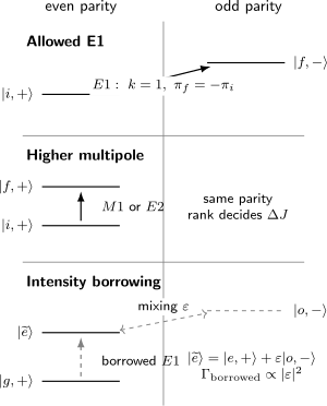
“Forbidden” always refers to a specified operator and model. An $E1$ line connects opposite parity at leading order; $M1$ and $E2$ can connect same-parity levels; and a perturbation can admix an opposite-parity component with amplitude $\varepsilon$, producing an $E1$ rate that is typically proportional to $|\varepsilon|^2$.

Polarization and Magnetic-Sublevel Rules

Choose a quantization axis and define spherical basis vectors by

$$\mathbf e_0=\mathbf e_z, \qquad \mathbf e_{\pm1} = \mp\frac{ \mathbf e_x\pm i\mathbf e_y }{\sqrt2}.$$

The scalar product of two vectors is

$$\mathbf d\mathbin{\cdot}\boldsymbol\epsilon = \sum_{q=-1}^{1} (-1)^q d_q\epsilon_{-q}.$$

For a transition driven by the operator component $T_q^{(k)}$,

$$\Delta M=q.$$

In the common atomic convention:

Operator component	Polarization label	Projection change
$q=0$	$\pi$	$\Delta M=0$
$q=+1$	$\sigma^+$	$\Delta M=+1$
$q=-1$	$\sigma^-$	$\Delta M=-1$

The association between $\sigma^\pm$ and photon helicity depends on propagation direction, absorption versus emission, and active-versus-passive conventions. The invariant statement is the value of $q$ used in the matrix element.

Linear polarization parallel to the quantization axis is pure $\pi$. Linear polarization perpendicular to that axis is a coherent superposition of $\sigma^+$ and $\sigma^-$. Circular polarization about the quantization axis selects one spherical component, subject to the convention just stated.

For fixed $M_i,M_f,q$, the relative angular strength is

$$\begin{aligned} S_q(M_i,M_f) \propto{}& \left| \begin{pmatrix} J_f & k & J_i\\ -M_f & q & M_i \end{pmatrix} \right|^2 \\ &\times \left| \langle \gamma_fJ_f \|T^{(k)}\| \gamma_iJ_i\rangle \right|^2 . \end{aligned}$$

The rule $\Delta M=q$ is necessary but not sufficient: an individual $3j$ coefficient can still vanish. For a rank-$1$ transition with $J_f=J_i$, for example, the $M=0\to M'=0$ component vanishes.

Polarization can also create nearly closed cycling transitions. Repeated $\sigma^+$ absorption on a suitable $F\to F+1$ line optically pumps population toward a stretched state. Closure is only as good as the level model: off-resonant hyperfine excitation, polarization impurity, magnetic-field misalignment, collisions, or decay to other manifolds creates leakage.

Forbidden Transitions and Metastable States

A state is metastable when every energetically open decay channel is suppressed enough to produce a long lifetime. Its total width is a sum over all radiative and nonradiative channels:

$$\begin{aligned} \Gamma_i ={}& \Gamma_i^{\mathrm{rad}} +\Gamma_i^{\mathrm{coll}} \\ &+\Gamma_i^{\mathrm{field}} +\cdots, \\ \Gamma_i^{\mathrm{rad}} ={}& \sum_f A_{if}^{E1} +\sum_f A_{if}^{M1} \\ &+\sum_f A_{if}^{E2} +\cdots . \end{aligned}$$

and

$$\tau_i=\Gamma_i^{-1}.$$

No single selection rule fixes $\tau_i$. A channel that is tiny compared with an allowed optical $E1$ rate may still dominate when all faster channels vanish.

Three examples expose different mechanisms:

• Hydrogen $2s\to1s$: one-photon $E1$ decay is forbidden because both states have even parity and $\Delta\ell=0$. The level decays mainly through a second-order two-photon $E1$–$E1$ process, giving a lifetime of about $0.12\ \mathrm{s}$ in isolated hydrogen.
• Ionic $S\leftrightarrow D$ clock lines: the same-parity $E1$ amplitude vanishes, but an $E2$ matrix element can drive the transition and set the radiative lifetime.
• Alkaline-earth-like $^1S_0\leftrightarrow{}^3P_0$ clock lines: the leading $E1$ amplitude is blocked by $J=0\leftrightarrow0$ and, in a pure $LS$ picture, by $\Delta S\ne0$. In fermionic isotopes, hyperfine mixing weakly opens the clock transition; in bosonic isotopes, controlled magnetic-field mixing can be used.

Metastability is environment dependent. Collisions can quench a state, blackbody radiation can transfer population, electric fields can mix parity, and a probe can power broaden or depopulate the level. A vacuum lifetime and an observed trap lifetime need not be the same.

How Perturbations Open a Forbidden Line

Suppose a perturbation $W$ admixes other field-free states into the initial level:

$$|\widetilde i\rangle = |i\rangle + \sum_{a\ne i} \frac{ \langle a|W|i\rangle }{ E_i-E_a } |a\rangle +\cdots.$$

A corresponding expression holds for $|\widetilde f\rangle$. The dressed transition amplitude becomes

$$\begin{aligned} \langle\widetilde f|T|\widetilde i\rangle \simeq{}& \langle f|T|i\rangle \\ &+ \sum_a \frac{ \langle f|T|a\rangle \langle a|W|i\rangle }{ E_i-E_a } \\ &+ \sum_b \frac{ \langle f|W|b\rangle \langle b|T|i\rangle }{ E_f-E_b }. \end{aligned}$$

If the unperturbed amplitude is zero but one admixture has size $\varepsilon$ and connects through an ordinary allowed matrix element, then

$$\mathcal M_{\mathrm{borrowed}} \sim \varepsilon\mathcal M_{\mathrm{allowed}},$$

so the borrowed rate is typically

$$\Gamma_{\mathrm{borrowed}} \sim |\varepsilon|^2 \Gamma_{\mathrm{allowed}}.$$

Small energy denominators can make the mixing much larger than a naive perturbation estimate. In that regime, diagonalize the coupled subspace and compute matrix elements between the actual eigenvectors.

Important mechanisms include:

Mixing or new process	What changes	Typical consequence
spin–orbit coupling	mixes nominal spin terms with the same $J,\pi$	intercombination lines acquire $E1$ strength
configuration interaction	mixes configurations with common exact labels	weak lines borrow oscillator strength
hyperfine interaction	mixes electronic $J$ character while coupling to $I$	hyperfine-induced clock transitions
static electric field	mixes opposite parity	parity-forbidden $E1$ amplitudes appear
magnetic field	mixes $J$ or $F$ but preserves parity	angular rules based on unmixed labels weaken
collisions or anisotropic environment	reduces isolated-atom symmetry and adds decay	quenching and pressure-induced lines
finite-wavelength terms	introduces $M1$, $E2$, and higher multipoles	one-photon decay beyond $E1$
two-photon coupling	uses a second-order composite amplitude	transitions such as hydrogen $2s\to1s$

The rule has not mysteriously failed. Either the eigenstates, the interaction operator, or the symmetry of the full problem has changed.

Reading and Predicting Atomic Spectra

Selection rules are one layer of a complete spectral model. To assign or predict a line:

1. Determine the element, isotope, ionization stage, configuration, parity, and best available angular-momentum labels.
2. Use measured or calculated level energies to locate candidate transitions.
3. Identify every operator relevant at the target sensitivity.
4. Evaluate $3j$ and, for recoupled states, $6j$ factors instead of relying only on shorthand $\Delta$ rules.
5. Obtain reduced matrix elements or critically evaluated transition probabilities with uncertainties.
6. Include field-induced mixing and track the field-dressed eigenvectors.
7. Model populations, branching, polarization, optical pumping, saturation, and line shape before comparing with intensity.

The NIST Atomic Spectra Database provides critically compiled wavelengths, classifications, transition probabilities, oscillator strengths, accuracy grades, and bibliographic links where available. Its option to generate possible Ritz $E1$ lines uses strict opposite-parity and $J$ rules, but a symmetry-allowed Ritz candidate is not a prediction of observable intensity. The reduced matrix element and experimental conditions still matter.

Applications to Atomic Spectra gives the shorter symmetry-first workflow. Spectroscopy owns apparatus and line interpretation, while Selection Rules in Spectroscopy compares atomic, rotational, vibrational, infrared, and Raman rules inside one measurement workflow.

Common Mistakes

Saying “forbidden” without naming the operator

A transition can be forbidden for $E1$ and allowed for $M1$, $E2$, or a two-photon process. Always attach the mechanism.

Replacing the triangle condition by a change rule

$|\Delta J|\leq k$ is necessary but incomplete. Check $|J_f-J_i|\leq k\leq J_f+J_i$, especially for $J=0$ and $J=1/2$.

Treating one-electron rules as exact many-electron symmetries

$\Delta\ell=\pm1$ is useful in a one-active-electron $E1$ picture. Correlated atomic eigenstates are superpositions of configurations, and their exact labels are total $J$ and parity.

Forgetting that spin rules depend on coupling

$\Delta S=0$ assumes a spin-independent electric dipole and nearly pure $LS$ terms. Spin–orbit and configuration mixing produce weak intercombination amplitudes.

Mapping helicity to a sign without a convention

The sign assigned to $\sigma^\pm$ can depend on propagation and emission-versus-absorption conventions. State the spherical operator component $q$.

Equating allowed with strong

An allowed angular coefficient can multiply a tiny radial integral or a cancellation. Frequency, branching, and populations also affect an observed line.

Equating metastable with stable

A metastable state has a small total width, not zero width. Higher multipoles, multiphoton decay, collisions, blackbody transfer, and field quenching remain.

Applying zero-field labels through a crossover

When a field mixes $F$, $J$, or parity, compute transitions between field-dressed eigenstates. Extrapolating a field-free rule through an avoided crossing can miss both new lines and vanished strengths.

Exercises

Exercise 1: Name the mechanism

Classify each transition at leading one-photon order: hydrogen $1s\to2p$, hydrogen $1s\to2s$, an atomic $J=0\to J'=0$ opposite-parity line, and a one-electron $S_{1/2}\to D_{5/2}$ same-parity line. State whether $E1$, $M1$, or $E2$ is allowed by rank and parity.

Solution

For hydrogen $1s\to2p$, parity changes and $\Delta\ell=1$, so $E1$ is allowed.

For hydrogen $1s\to2s$, the states have the same parity and $\Delta\ell=0$. $E1$ is forbidden. A single-photon $M1$ amplitude is also absent in the leading nonrelativistic model because the radial and angular structure does not connect these two $S$ states; the observed decay proceeds mainly by two-photon emission.

For opposite-parity $J=0\to J'=0$, parity is suitable for $E1$, but a rank-$1$ operator cannot connect two $J=0$ states. $M1$ has the same rank problem and also the wrong parity. $E2$ has the wrong parity and its rank-$2$ triangle condition also excludes $0\to0$.

For $S_{1/2}\to D_{5/2}$, the states have the same parity. $E1$ is forbidden. $M1$ has even parity but rank $1$, so $J=1/2\to5/2$ is excluded. $E2$ has even parity and satisfies

$$\left|\frac52-\frac12\right| =2 \leq2 \leq3,$$

so it is allowed by rank and parity.

Exercise 2: Polarization from a scalar initial state

An $E1$ transition starts from $J_i=0,M_i=0$ and ends in $J_f=1$. Which final $M_f$ is driven by each operator component $q=0,+1,-1$? Are the three components distinguished by reduced atomic dynamics?

Solution

The projection rule gives

$$M_f=M_i+q=q.$$

Thus $q=0$ drives $M_f=0$, $q=+1$ drives $M_f=+1$, and $q=-1$ drives $M_f=-1$. All three share the same reduced matrix element

$$\langle \gamma_f,J_f=1 \|d^{(1)}\| \gamma_i,J_i=0\rangle.$$

Rotational symmetry makes their reduced dynamics identical. Their laboratory excitation strengths differ only through the available field polarization and geometry; with equal pure spherical-component amplitudes, the three $3j$ coefficients have equal magnitude.

Exercise 3: Hyperfine branches

An isotope has $I=3/2$ and an electronic transition $J_i=1/2\to J_f=1/2$. The initial hyperfine level is $F_i=1$. List the $F_f$ values that exist and identify which satisfy the $E1$ hyperfine rule.

Solution

Coupling $J_f=1/2$ to $I=3/2$ gives

$$F_f=|I-J_f|,\ldots,I+J_f=1,2.$$

From $F_i=1$, the rank-$1$ rule permits $\Delta F=0,\pm1$, excluding only $0\leftrightarrow0$. Both existing final values,

$$\begin{gathered} F_i=1\to F_f=1,\\ F_i=1\to F_f=2. \end{gathered}$$

are therefore allowed by hyperfine angular momentum. Their relative strengths require the relevant $6j$ factors and the common reduced electronic matrix element.

Exercise 4: Intensity borrowing

A perturbation admixes an $E1$-allowed opposite-parity state into a nominally forbidden upper state with amplitude $\varepsilon=2\times10^{-3}$. Neglect interference and other channels. Estimate the borrowed rate as a fraction of the fully allowed rate.

Solution

The borrowed amplitude is approximately

$$\mathcal M_{\mathrm b} \simeq \varepsilon\mathcal M_{\mathrm a}.$$

Rates are proportional to squared amplitudes, so

$$\frac{\Gamma_{\mathrm b}} {\Gamma_{\mathrm a}} \simeq |\varepsilon|^2 = 4\times10^{-6}.$$

A part-per-thousand state admixture can therefore create a part-per-million radiative rate relative to an otherwise comparable allowed line.

Exercise 5: A quenched metastable lifetime

An isolated metastable state has an $E2$ decay rate $0.80\ \mathrm{s}^{-1}$ and all other vacuum channels total $0.05\ \mathrm{s}^{-1}$. In a buffer gas, collisions add a quenching rate $0.15\ \mathrm{s}^{-1}$. Find the vacuum and buffer-gas lifetimes.

Solution

In vacuum,

$$\Gamma_{\mathrm{vac}} = 0.80+0.05 = 0.85\ \mathrm{s}^{-1},$$

so

$$\tau_{\mathrm{vac}} = \frac{1}{0.85\ \mathrm{s}^{-1}} \simeq1.18\ \mathrm{s}.$$

With collisional quenching,

$$\Gamma_{\mathrm{gas}} = 0.85+0.15 = 1.00\ \mathrm{s}^{-1},$$

and $\tau_{\mathrm{gas}}=1.00\ \mathrm{s}$. Selection-rule suppression of fast radiative channels does not protect the state from environmental decay.

Exercise 6: Use the full rank-2 triangle

For an $E2$ operator, classify the angular-momentum pairs $1/2\to1/2$, $1/2\to3/2$, $0\to1$, and $0\to2$ using the full triangle condition.

Solution

For rank $k=2$, require

$$|J_f-J_i| \leq2 \leq J_f+J_i.$$

For $1/2\to1/2$, the upper bound is $J_f+J_i=1$, so the transition is excluded. For $1/2\to3/2$, the bounds are $1\leq2\leq2$, so it is allowed by angular momentum. For $0\to1$, the upper bound is $1$, so it is excluded. For $0\to2$, both bounds equal $2$, so it is allowed.

This exercise shows why the shorthand $\Delta J=0,\pm1,\pm2$ is unsafe at small $J$.

Cross-Links

• Atomic Physics
• Atomic Orbitals Revisited
• Alkali Atoms
• Atomic Term Symbols
• LS Coupling
• Fine Structure
• Hyperfine Structure
• Zeeman Effect in Atoms
• Stark Effect in Atoms
• Wigner–Eckart Theorem
• Selection Rules
• Parity Selection Rules
• Dipole Transitions
• Multipole Operators
• Applications to Atomic Spectra
• Selection Rules in Transition Rates
• Selection Rules in Spectroscopy
• Selection Rule Tables for a compact E1, M1, E2, polarization, and molecular lookup
• Oscillator Strength Reference for the E1 strength, degeneracy, and sum-rule ledger
• Spectroscopy
• AMO Physics Roadmap

References

1. E. U. Condon and G. H. Shortley, The Theory of Atomic Spectra, Cambridge University Press, 1935.
2. I. I. Sobelman, Atomic Spectra and Radiative Transitions, 2nd ed., Springer, 1992.
3. R. D. Cowan, The Theory of Atomic Structure and Spectra, University of California Press, 1981.
4. W. R. Johnson, Atomic Structure Theory: Lectures on Atomic Physics, Springer, 2007.
5. C. J. Foot, Atomic Physics, Oxford University Press, 2005.
6. C. Cohen-Tannoudji, J. Dupont-Roc, and G. Grynberg, Atom–Photon Interactions: Basic Processes and Applications, Wiley, 1992.
7. A. R. Edmonds, Angular Momentum in Quantum Mechanics, Princeton University Press, 1957.
8. W. C. Martin and W. L. Wiese, “Atomic Spectroscopy: An Introduction,” in G. W. F. Drake, ed., Atomic, Molecular, and Optical Physics Handbook, AIP Press, 1996.
9. A. Kramida, Yu. Ralchenko, J. Reader, and the NIST ASD Team, NIST Atomic Spectra Database, version 5.12, National Institute of Standards and Technology, 2024, DOI: 10.18434/T4W30F, accessed 2026-07-21.
10. M. Göppert-Mayer, “Über Elementarakte mit zwei Quantensprüngen,” Annalen der Physik 401, 273–294 (1931), DOI: 10.1002/andp.19314010303.
11. S. G. Porsev and A. Derevianko, “Hyperfine quenching of the metastable $^3P_{0,2}$ states in divalent atoms,” Physical Review A 69, 042506 (2004), DOI: 10.1103/PhysRevA.69.042506.
12. G. W. F. Drake, ed., Springer Handbook of Atomic, Molecular, and Optical Physics, 2nd ed., Springer, 2006.
13. M. E. Rose, Elementary Theory of Angular Momentum, Wiley, 1957.
14. H. Friedrich, Theoretical Atomic Physics, 4th ed., Springer, 2017.