Multipole Expansion

The multipole expansion organizes how a localized charge and current distribution exchanges energy, momentum, and angular momentum with an electromagnetic field. Electric-dipole coupling, E1, is only its leading term. Magnetic-dipole M1, electric-quadrupole E2, and higher multipoles become essential when E1 is forbidden, accidentally small, suppressed by mode geometry, or inadequate at the target precision.

For a neutral system expanded about $\mathbf R$, the first local interactions are

$$\begin{aligned} H_{\mathrm{int}} ={}& - \mathbf d \mathbin{\cdot} \mathbf E(\mathbf R) \\ &- \boldsymbol\mu \mathbin{\cdot} \mathbf B(\mathbf R) \\ &- \frac{1}{6} \Theta_{ij} \partial_i E_j(\mathbf R) + \cdots. \end{aligned}$$

Here $\boldsymbol\mu$ is the magnetic dipole and $\Theta_{ij}$ is the traceless electric quadrupole in the convention defined below. The three terms sample different local features of the same mode: electric field, magnetic field, and electric-field gradient.

The expansion is useful only when two ideas are kept separate:

• Multipole order classifies interaction amplitudes by spatial structure and radiation symmetry.
• Perturbative order counts powers of the interaction in a transition process.

An E2 transition is first order in a weak applied field but subleading in the spatial multipole expansion. A two-photon E1–E1 transition is second order in the field interaction but uses E1 operators at each vertex.

Canonical Scope

This page owns the AMO dynamics of the multipole hierarchy:

1. how E1, M1, E2, and higher terms couple to local fields;
2. how their amplitudes and spontaneous rates scale;
3. how standing waves, focused beams, and near fields select different terms;
4. how weak one-photon channels create metastable states;
5. why narrow M1, E2, and E3 lines are useful, but not automatically ideal, for precision spectroscopy.

Dipole Approximation owns the controlled Taylor expansion, transition-density length scale, origin bookkeeping, and center-of-mass distinction. Multipole Operators owns the derivation of tensor rank and parity. Atomic Selection Rules applies those rules to electronic, fine, and hyperfine labels.

The purpose here is not to duplicate those derivations. It is to connect the operators to fields, matrix elements, rates, lifetimes, and experimental choices.

From Spatial Coupling to Multipoles

Plane-wave expansion

For an internal coordinate $\boldsymbol\rho$ and a plane-wave component,

$$e^{i\mathbf k\cdot( \mathbf R+\boldsymbol\rho )} = e^{i\mathbf k\cdot\mathbf R} e^{i\mathbf k\cdot\boldsymbol\rho}.$$

The internal factor expands as

$$\begin{aligned} e^{i\mathbf k\cdot\boldsymbol\rho} ={}& 1 + i\mathbf k \mathbin{\cdot} \boldsymbol\rho \\ &- \frac{1}{2} \left( \mathbf k \mathbin{\cdot} \boldsymbol\rho \right)^2 + \cdots. \end{aligned}$$

Charge and current conservation reorganize these powers into electric and magnetic multipoles. A consistent first correction to E1 contains both M1 and E2. Keeping one arbitrarily selected Cartesian Taylor term is not generally equivalent to keeping a complete multipole order.

The center-of-mass phase

$$e^{i\mathbf k\cdot\mathbf R}$$

is not part of the internal multipole truncation. It can still produce recoil, Doppler shifts, and motional sidebands.

Spherical-wave viewpoint

An exact radiation field about an origin can also be decomposed into electric and magnetic spherical multipoles. Their radial dependence contains spherical Bessel functions. At small argument,

$$\begin{aligned} j_\lambda(z) &= \frac{ z^\lambda }{ (2\lambda+1)!! } \\ &\quad\times \left[ 1-\frac{z^2}{2(2\lambda+3)}+\cdots \right]. \end{aligned}$$

This small-$kr$ behavior generates the long-wavelength hierarchy. For typical nonzero electric moments,

$$\frac{ \mathcal A(E\lambda) }{ \mathcal A(E1) } \sim (ka)^{\lambda-1}.$$

Magnetic moments contain internal currents. A common nonrelativistic estimate is

$$\frac{ \mathcal A(M1) }{ \mathcal A(E1) } \sim \frac{v}{c},$$

when both comparison amplitudes are allowed and have otherwise comparable structure. Neither estimate is a selection rule. A zero E1 denominator means a higher multipole must be compared with the leading nonzero amplitude instead.

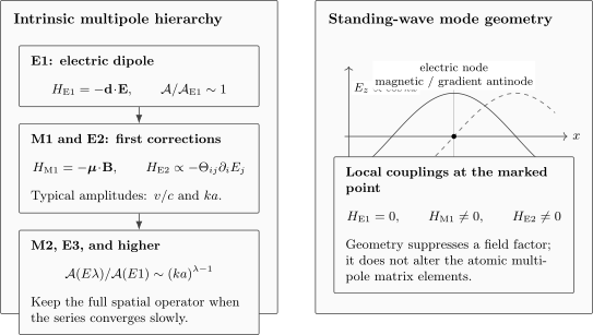
Multipole order and mode geometry are independent filters. In a standing wave, an electric-field node suppresses local E1 coupling while the magnetic field and electric gradient can be maximal, making M1 or E2 experimentally accessible without changing the intrinsic atomic selection rules.

Gauge, origin, and truncation

The exact minimal-coupling and multipolar theories are unitarily related when states, observables, self-energy terms, and boundary conditions are transformed together. Their truncated pieces need not agree term by term.

An origin shift also mixes Cartesian multipole coefficients. Observable amplitudes remain origin independent when all contributions through the claimed order are retained. Beyond E1, this includes interference terms in the probability, not only squares of selected M1 or E2 amplitudes.

These issues are developed in Gauge Choices in Light–Matter Physics and Dipole Approximation.

Electric Dipole E1

Coupling and matrix element

The leading electric interaction is

$$H_{E1} = - \mathbf d \mathbin{\cdot} \mathbf E(\mathbf R), \qquad \mathbf d = \sum_a q_a\boldsymbol\rho_a.$$

For a transition $|i\rangle\to|f\rangle$,

$$\mathcal M_{fi}^{E1} = - \mathbf d_{fi} \mathbin{\cdot} \mathbf E(\mathbf R), \qquad \mathbf d_{fi} = \langle f|\mathbf d|i\rangle.$$

E1 samples the electric field itself. In a freely propagating optical mode, it usually dominates allowed transitions because it carries no additional internal factor of $ka$ or $v/c$.

Spontaneous rate

For a vacuum transition with angular frequency $\omega_{if}>0$, the polarization- and direction-summed E1 rate can be written

$$A_{i\to f}^{E1} = \frac{ \omega_{if}^3 }{ 3\pi\epsilon_0\hbar c^3 } \frac{ S(E1) }{ 2J_i+1 },$$

where the line strength in the stated reduced-matrix-element convention is

$$S(E1) = \left| \langle \gamma_fJ_f \| \mathbf d^{(1)} \| \gamma_iJ_i \rangle \right|^2.$$

The factor $1/(2J_i+1)$ averages over an unresolved upper magnetic manifold. For a prepared $M_i$ state or a restricted photonic environment, one must sum the resolved angular and polarization channels instead.

The $\omega^3$ factor contains both the field amplitude per photon and the three-dimensional photon density of states. A matrix element alone does not set a lifetime.

Canonical handoff

The spatial validity of E1 lives in Dipole Approximation. The E1 rank, parity, and polarization rules live in Dipole Transitions. The conversion of matrix elements into absorption, stimulated emission, and spontaneous emission lives in Transition Rates in Light–Matter Interaction.

Magnetic Dipole M1

Magnetic moment operator

The M1 interaction is

$$H_{M1} = - \boldsymbol\mu \mathbin{\cdot} \mathbf B(\mathbf R).$$

For nonrelativistic particles with orbital and spin angular momenta, a schematic magnetic moment is

$$\boldsymbol\mu = \sum_a \frac{q_a}{2m_a} \left( \mathbf L_a + g_a\mathbf S_a \right).$$

For an electron,

$$\boldsymbol\mu_e \simeq - \frac{\mu_B}{\hbar} \left( \mathbf L + g_s\mathbf S \right), \qquad \mu_B = \frac{e\hbar}{2m_e}.$$

Relativistic, anomalous-moment, nuclear, and many-electron corrections are added according to the required accuracy.

Unlike $\mathbf d$, the magnetic dipole is an axial vector. M1 therefore has rank $1$ but even parity. This makes it a common channel between same-parity fine-structure or hyperfine levels.

Field scale and E1 comparison

For a plane wave in vacuum,

$$|\mathbf B| = \frac{|\mathbf E|}{c}.$$

The same-field amplitude comparison is therefore

$$\frac{ |\mathcal M^{M1}| }{ |\mathcal M^{E1}| } \sim \frac{ |\mu_{fi}| }{ c|d_{fi}| }.$$

Using characteristic electronic moments

$$|\mu_{fi}| \sim \mu_B, \qquad |d_{fi}| \sim ea_0,$$

gives

$$\frac{ \mu_B }{ cea_0 } = \frac{\alpha}{2} \simeq 3.65\times10^{-3}.$$

The corresponding rate suppression is roughly

$$\left( \frac{\alpha}{2} \right)^2 \simeq 1.33\times10^{-5}$$

at the same frequency and for comparable angular factors. Real matrix elements can differ by orders of magnitude.

Spontaneous rate

With the analogous reduced magnetic line strength

$$S(M1) = \left| \langle \gamma_fJ_f \| \boldsymbol\mu^{(1)} \| \gamma_iJ_i \rangle \right|^2,$$

the free-space rate is

$$A_{i\to f}^{M1} = \frac{ \mu_0\omega_{if}^3 }{ 3\pi\hbar c^3 } \frac{ S(M1) }{ 2J_i+1 }.$$

M1 and E1 share the $\omega^3$ phase-space scaling. The enormous lifetime of a low-frequency M1 line can therefore come from frequency as well as from its magnetic matrix element.

The hydrogen ground-state hyperfine transition near $21\ \mathrm{cm}$ is a canonical example. It is M1 allowed, but its gigahertz frequency makes its vacuum spontaneous rate extremely small compared with an optical transition of similar dimensionless angular strength.

Mode geometry

M1 responds to $\mathbf B(\mathbf R)$, not to the electric field. In a traveling plane wave, the two are locked by Maxwell’s equations. In a standing wave, cavity, waveguide, or near field, their local nodes and antinodes can differ. Placing a system near an electric node can suppress E1 while retaining M1.

The magnetic field also chooses spherical components relative to the quantization axis. A statement such as “M1 is allowed” is incomplete until the field orientation and addressed magnetic sublevels are specified.

Electric Quadrupole E2

Quadrupole conventions

Define the primitive second moment

$$M_{ij} = \sum_a q_a \rho_{a,i}\rho_{a,j}.$$

Its interaction with a smooth electric field is

$$H_{E2} = - \frac{1}{2} M_{ij} \partial_iE_j(\mathbf R).$$

A common traceless quadrupole is

$$\Theta_{ij} = \sum_a q_a \left( 3\rho_{a,i}\rho_{a,j} - \rho_a^2\delta_{ij} \right).$$

In a source-free region,

$$\boldsymbol\nabla \mathbin{\cdot} \mathbf E = 0,$$

so the same interaction becomes

$$H_{E2} = - \frac{1}{6} \Theta_{ij} \partial_iE_j(\mathbf R).$$

The coefficients $1/2$ and $1/6$ refer to different tensor definitions. Quoting an E2 matrix element without its convention is insufficient.

Gradient coupling

For a plane wave,

$$\partial_i E_j = ik_iE_j.$$

The E2 transition amplitude is therefore

$$\mathcal M_{fi}^{E2} = - \frac{i}{6} k_iE_j \left( \Theta_{ij} \right)_{fi}.$$

With

$$|\Theta_{fi}| \sim |d_{fi}|a,$$

one obtains the usual scale estimate

$$\frac{ |\mathcal M^{E2}| }{ |\mathcal M^{E1}| } \sim ka$$

when the E1 denominator is nonzero. The E2 rate is then typically suppressed by $(ka)^2$ relative to a comparable E1 line at the same frequency.

E2 samples the symmetric rank-$2$ part of the electric-field gradient. A large scalar gradient estimate does not guarantee coupling to a chosen tensor component; atomic orientation, polarization, propagation direction, and magnetic sublevels all matter.

Same parity and rank two

E2 is parity even and has rotational rank $2$. It can therefore connect same-parity levels with angular separations inaccessible to E1 or M1. The $S_{1/2}\leftrightarrow D_{5/2}$ transition in $^{40}\mathrm{Ca}^{+}$ near $729\ \mathrm{nm}$ is a standard E2 example.

The complete rank-$2$ triangle and projection rules live in Multipole Operators and their atomic application in Atomic Selection Rules.

Standing-wave and near-field enhancement

At a standing-wave electric node,

$$\mathbf E(\mathbf R) = 0$$

while

$$\boldsymbol\nabla\mathbf E(\mathbf R) \ne 0.$$

The local E1 drive then vanishes while E2 can remain finite. This does not make the intrinsic E2 matrix element larger. It changes the field factor multiplying each operator.

Nanophotonic and near-field structures can provide gradients on scales shorter than the free-space wavelength. The relevant expansion parameter is then $a/L_E$, and the full mode profile must satisfy Maxwell boundary conditions. A gradient enhancement should be compared with loss, surface noise, modified spontaneous emission, and breakdown of a low-order expansion.

Transition quadrupole versus static quadrupole

The off-diagonal quantity

$$\left( \Theta_{ij} \right)_{fi}$$

drives an E2 transition. The diagonal quantity

$$\left( \Theta_{ij} \right)_{ii}$$

is a static quadrupole moment and can shift a level in a static electric gradient.

These are different matrix elements. An E2 clock transition does not by itself prove that the clock shift has a nonzero static quadrupole moment, and a state with a static quadrupole can participate in a transition of another multipolarity. Clock systematics must be evaluated state by state.

Higher Multipoles

Electric moments

A spherical electric multipole operator can be defined as

$$\begin{aligned} Q_q^{(\lambda)} &= \sum_a q_a \rho_a^\lambda C_q^{(\lambda)} \left( \widehat{\boldsymbol\rho}_a \right), \\ q &= -\lambda,\ldots,\lambda. \end{aligned}$$

where

$$C_q^{(\lambda)} = \sqrt{ \frac{ 4\pi }{ 2\lambda+1 } } Y_\lambda^q.$$

It has rank $\lambda$ and parity $(-1)^\lambda$. E3 is the electric octupole, E4 the electric hexadecapole, and so on.

For comparable electric structure,

$$\mathcal A(E1): \mathcal A(E2): \mathcal A(E3) \sim 1: ka: (ka)^2.$$

The corresponding rate hierarchy is nominally

$$1: (ka)^2: (ka)^4,$$

before matrix-element, frequency, and angular factors are included.

Magnetic moments

Magnetic multipoles are current and magnetization moments. M2 has rank $2$ and odd parity; M3 has rank $3$ and even parity. Their exact operators are more model dependent than the charge-only electric moments because convection current, spin magnetization, relativistic corrections, and many-body currents can all contribute.

The robust labels are

$$\begin{aligned} \operatorname{parity}(E\lambda) &= (-1)^\lambda, \\ \operatorname{parity}(M\lambda) &= (-1)^{\lambda+1}. \end{aligned}$$

Electric octupole clock line

The $^{171}\mathrm{Yb}^{+}$ transition

$${}^2S_{1/2} \longleftrightarrow {}^2F_{7/2}$$

near $467\ \mathrm{nm}$ is E3. Its suppression produces an exceptionally long excited-state lifetime. A direct measurement reported

$$\tau = 4.98(25)\times10^7\ \mathrm{s},$$

about $1.58$ years. The same weakness that yields a tiny natural linewidth requires substantial probe intensity or long coherent interrogation and creates sensitivity to probe-induced Stark shifts.

Electric monopole is not a one-photon line

E0 has rank $0$ and even parity, but a real transverse photon cannot carry zero total angular momentum about the emission origin. Charge conservation also prevents a time-dependent total monopole charge in an isolated atomic transition.

An E0 matrix element can matter in nuclear internal conversion or pair creation when energetically allowed, and scalar operators can contribute in collisions or other probes. It does not describe ordinary single-real-photon atomic emission.

Higher multipole versus multiphoton

An E3 transition is one-photon coupling through a rank-$3$ operator. A two-photon E1–E1 process contains two rank-$1$ vertices and intermediate state denominators. They can obey different angular, parity, intensity, and frequency rules.

For example, hydrogen $2s\to1s$ decays mainly by two-photon E1–E1 emission, not by relabeling the transition as a high one-photon multipole.

When to keep the full spatial operator

If

$$ka \gtrsim 1,$$

many multipoles can contribute and the hierarchy can converge slowly. Retaining the exact $e^{i\mathbf k\cdot\boldsymbol\rho}$ dependence or the full current–field interaction is often safer than extending a truncated series to high order.

This is particularly relevant in X-ray spectroscopy, large molecules, Rydberg and continuum processes, and strongly structured near fields.

Selection-Rule Summary

For an irreducible multipole of rank $\lambda$, the exact angular condition is

$$|J_f-J_i| \le \lambda \le J_f+J_i.$$

Its spherical component fixes

$$M_f-M_i = q, \qquad q=-\lambda,\ldots,\lambda.$$

If the states have definite parity,

$$\pi_f\pi_i = \begin{cases} (-1)^\lambda, & E\lambda, \\ (-1)^{\lambda+1}, & M\lambda. \end{cases}$$

The most common one-photon cases are:

Type	Rank	Parity relation	Field sampled
E1	$1$	opposite	$\mathbf E$
M1	$1$	same	$\mathbf B$
E2	$2$	same	rank-$2$ part of $\boldsymbol\nabla\mathbf E$
M2	$2$	opposite	magnetic gradient
E3	$3$	opposite	second electric gradient

These are necessary conditions, not strength predictions. A reduced matrix element can vanish because of configuration, spin, radial orthogonality, exchange symmetry, or cancellation.

Mixed M1 and E2 lines

M1 and E2 have the same parity and can both contribute when the angular triangle permits them. The amplitude for a resolved propagation direction and polarization is then

$$\mathcal A = \mathcal A_{M1} + \mathcal A_{E2} + \cdots.$$

Interference depends on geometry, state preparation, and what is integrated over. A database label such as M1+E2 means that one line strength without a specified decomposition is not sufficient.

State mixing

External fields, hyperfine coupling, spin–orbit coupling, and configuration interaction can admix states and open an E1 amplitude on a nominally forbidden line. That borrowed E1 amplitude can dominate a bare M1 or E2 channel even when the admixture is small.

The correct procedure is to diagonalize the stated Hamiltonian, evaluate all relevant operators between the dressed states, and compare amplitudes. Field-free labels remain useful descriptors, not exact rules, after strong mixing.

From Amplitudes to Rates

Frequency scaling

With a standard reduced line strength $S(X\lambda)$,

$$A_{i\to f}^{X\lambda} = \frac{ C_{X\lambda} \omega_{if}^{2\lambda+1} }{ 2J_i+1 } S(X\lambda),$$

where $X=E$ or $M$. The constant $C_{X\lambda}$ contains SI factors and depends on the normalization chosen for the multipole operator.

The robust frequency powers are:

Multipole	Frequency factor in the free-space rate
E1 or M1	$\omega^3$
E2 or M2	$\omega^5$
E3 or M3	$\omega^7$

This is why low-frequency fine-structure and hyperfine M1 lines can have very long lifetimes even when their dimensionless angular matrix elements are ordinary.

Lifetime and branching

For an upper state $i$,

$$\Gamma_i^{\mathrm{rad}} = \sum_f \sum_{X,\lambda} A_{i\to f}^{X\lambda}.$$

Including nonradiative and environment-induced channels,

$$\begin{aligned} \Gamma_i ={}& \Gamma_i^{\mathrm{rad}} + \Gamma_i^{\mathrm{coll}} + \Gamma_i^{\mathrm{field}} + \cdots, \\ \tau_i ={}& \frac{1}{\Gamma_i}. \end{aligned}$$

The branching fraction for one channel is

$$b_{i\to f}^{X\lambda} = \frac{ A_{i\to f}^{X\lambda} }{ \Gamma_i }.$$

“E2 lifetime” is meaningful only if E2 is known to dominate the complete width.

Stimulated driving is not set by A alone

A spontaneous rate characterizes coupling to the available vacuum modes. A coherent Rabi frequency depends on the applied local field:

$$\begin{aligned} \hbar\Omega_{E1} &\sim - \mathbf d_{fi} \mathbin{\cdot} \boldsymbol{\mathcal E}, \\ \hbar\Omega_{M1} &\sim - \boldsymbol\mu_{fi} \mathbin{\cdot} \boldsymbol{\mathcal B}, \\ \hbar\Omega_{E2} &\sim - \frac{1}{6} \left( \Theta_{ij} \right)_{fi} \partial_i\mathcal E_j. \end{aligned}$$

A cavity or nanophotonic structure can enhance selected field factors and modify the photonic density of states. The free-space lifetime is then not the whole dynamical model.

Database conventions

Atomic transition databases may tabulate $A$, oscillator strength, and line strength using different units and upper-level degeneracy factors. NIST, for example, uses distinct conversion constants for E1, M1, E2, M2, E3, and M3 and explicitly labels mixed M1+E2 lines.

Before converting a tabulated number:

1. identify whether the quoted wavelength is vacuum or air;
2. identify the upper and lower level convention;
3. check whether $g_iA$, $A$, $f$, or $S$ is tabulated;
4. check the units and multipole normalization;
5. use the uncertainty or accuracy grade rather than inventing precision.

Forbidden Transitions and Precision Clocks

Forbidden means operator specific

A line is never simply “forbidden.” It is forbidden for a named operator under stated symmetries. A same-parity $S\leftrightarrow D$ line can be E1 forbidden and E2 allowed. A $J=0\leftrightarrow0$ line can be forbidden for every one-photon multipole with positive rank yet opened by hyperfine mixing or a two-photon process.

The total observed line can contain:

• a bare M1, E2, or higher one-photon amplitude;
• an E1 amplitude borrowed through state mixing;
• a multiphoton amplitude;
• collision- or environment-induced coupling;
• several coherent amplitudes that interfere.

Narrowness and quality factor

For an isolated state with lifetime $\tau$ and lifetime-limited full width at half maximum,

$$\Delta\nu_{\mathrm{nat}} = \frac{ 1 }{ 2\pi\tau }.$$

The natural quality factor is

$$Q_{\mathrm{nat}} = \frac{ \nu_0 }{ \Delta\nu_{\mathrm{nat}} } = 2\pi\nu_0\tau.$$

Suppressing fast E1 decay can therefore produce enormous $Q$. In an actual clock, the observed linewidth may instead be limited by probe coherence, finite interrogation time, collisions, magnetic noise, or motion.

Representative mechanisms

• Hydrogen $21\ \mathrm{cm}$: an M1 hyperfine transition with strong $\omega^3$ suppression of spontaneous emission.
• $^{40}\mathrm{Ca}^{+}$ and $^{88}\mathrm{Sr}^{+}$ ion clocks: same-parity $S\leftrightarrow D$ E2 transitions.
• $^{171}\mathrm{Yb}^{+}$: an E2 clock transition near $436\ \mathrm{nm}$ and an E3 clock transition near $467\ \mathrm{nm}$ in the same ion.
• Fermionic alkaline-earth-like clocks: nominal $\,{}^1S_0\leftrightarrow{}^3P_0$ lines are enabled by hyperfine mixing; they should not be described as simply M1 or E2.
• Bosonic $J=0\leftrightarrow0$ clocks: controlled field-induced mixing or multiphoton schemes may open an otherwise forbidden line.

The clock tradeoff

A weaker transition offers:

• a long natural lifetime;
• a narrow natural linewidth;
• reduced spontaneous-emission decoherence during interrogation;
• high sensitivity of accumulated phase to frequency.

It can also require:

• higher probe intensity or longer pulses;
• tighter laser coherence;
• careful control of probe Stark shifts;
• accurate polarization and magnetic-field alignment;
• suppression of off-resonant coupling;
• long state-preparation and readout cycles.

Narrowness is necessary for many clock strategies but not sufficient for a small uncertainty budget.

Quadrupole shifts

An excited state with a nonzero static electric quadrupole moment couples to trap or environmental electric-field gradients. This can shift and inhomogeneously broaden an ion-clock transition:

$$\Delta E_Q \propto \left( \Theta_{ij} \right)_{ii} \partial_iE_j^{\mathrm{static}}.$$

Orientation averaging, averaging over Zeeman components, field-axis rotation, dynamical decoupling, or choosing states with vanishing tensor moments can suppress the shift. The required strategy depends on the actual state and apparatus.

Precision Spectroscopy owns the full observation equation, uncertainty, clock comparison, and systematic-shift workflow.

Worked Examples

E2 suppression for a visible atomic transition

Take

$$a = a_0, \qquad \lambda = 500\ \mathrm{nm}.$$

Then

$$ka \simeq 6.65\times10^{-4}.$$

For comparable nonzero internal moments and angular factors,

$$\frac{ |\mathcal A(E2)| }{ |\mathcal A(E1)| } \sim 6.7\times10^{-4},$$

and

$$\frac{ A(E2) }{ A(E1) } \sim 4.4\times10^{-7}.$$

If E1 is exactly zero, the second ratio is not a branching estimate. E2 can be the leading available channel despite its absolute smallness.

Frequency suppression of a magnetic-dipole line

Compare two hypothetical M1 lines with the same reduced matrix element, one at

$$\nu_{\mathrm{hf}} = 1.420\ \mathrm{GHz}$$

and one at

$$\nu_{\mathrm{opt}} = 5.00\times10^{14}\ \mathrm{Hz}.$$

Since $A(M1)\propto\nu^3$,

$$\begin{aligned} \frac{ A_{\mathrm{hf}} }{ A_{\mathrm{opt}} } &= \left( \frac{ \nu_{\mathrm{hf}} }{ \nu_{\mathrm{opt}} } \right)^3 \\ &\simeq 2.29\times10^{-17}. \end{aligned}$$

This comparison isolates phase space. Actual hyperfine and optical magnetic matrix elements need not be equal.

Standing-wave node

A Maxwell-consistent standing wave can be written

$$\begin{aligned} \mathbf E(x,t) &= \widehat{\mathbf z} E_0 \cos(kx) \cos(\omega t), \\ \mathbf B(x,t) &= - \widehat{\mathbf y} \frac{E_0}{c} \sin(kx) \sin(\omega t). \end{aligned}$$

At

$$kx = \frac{\pi}{2},$$

the electric field vanishes while

$$|\mathbf B| \quad\text{and}\quad \left| \partial_xE_z \right|$$

are maximal in space. E1 is locally suppressed, while M1 and E2 have nonzero field factors. Their temporal phases differ by a quarter cycle, so coherent interference also depends on timing and complex-amplitude conventions.

Lifetime from competing channels

Suppose a metastable level has

$$A_{M1} = 0.20\ \mathrm{s}^{-1}, \qquad A_{E2} = 0.75\ \mathrm{s}^{-1},$$

and a collision-induced quenching rate

$$\Gamma_{\mathrm{coll}} = 0.05\ \mathrm{s}^{-1}.$$

The total width is

$$\Gamma = 1.00\ \mathrm{s}^{-1},$$

so

$$\tau = 1.00\ \mathrm{s}.$$

The E2 branching fraction is

$$b_{E2} = \frac{0.75}{1.00} = 0.75.$$

The level is not an “E2-only” state even though E2 supplies the largest single channel.

Natural quality factor

For

$$\lambda = 729\ \mathrm{nm}, \qquad \tau = 1.0\ \mathrm{s},$$

the optical frequency is

$$\nu_0 = \frac{c}{\lambda} \simeq 4.11\times10^{14}\ \mathrm{Hz}.$$

The lifetime-limited linewidth and quality factor are

$$\Delta\nu_{\mathrm{nat}} \simeq 0.159\ \mathrm{Hz},$$ $$Q_{\mathrm{nat}} \simeq 2.58\times10^{15}.$$

This is a natural limit, not a guarantee that a laboratory interrogation will resolve a $0.159\ \mathrm{Hz}$ line.

A Practical Multipole Workflow

1. Name the observable. Total lifetime, directional emission, polarization asymmetry, coherent Rabi rate, and clock shift require different sums and interference terms.
2. Choose the parent interaction. State the gauge or representation, expansion point, dynamical center-of-mass variables, and field quantization.
3. Check the spatial expansion. Estimate $ka$ and local gradient scales over the relevant transition charge and current distributions.
4. List candidate operators. Include E1, M1, E2, higher multipoles, state mixing, and multiphoton channels allowed at the target precision.
5. Apply exact symmetry first. Use full triangle, projection, parity, exchange, and field-dressed labels.
6. Evaluate matrix elements. “Allowed” is not a numerical estimate.
7. Insert the actual mode. Evaluate $\mathbf E$, $\mathbf B$, and gradients at the system, including polarization and orientation.
8. Expand probabilities consistently. Retain cross terms through the claimed order and test origin stability.
9. Compute the complete width. Add every radiative, collisional, and environment-induced channel before quoting a lifetime or branching ratio.
10. Converge or abandon the truncation. If multipole order converges slowly, compare with the full spatial interaction.

Common Mistakes

• Calling a transition “forbidden” without naming E1, M1, E2, or another process.
• Treating multipole order as perturbative order in the field.
• Assuming $ka\ll1$ guarantees E1 dominance.
• Using $\mathbf B=\mathbf E/c$ locally inside a standing wave, cavity, or near field without checking the mode.
• Omitting M1 when keeping E2 as the first correction to E1.
• Comparing quadrupole formulas that use different primitive, traceless, or spherical normalizations.
• Confusing an off-diagonal E2 transition moment with a diagonal static quadrupole moment.
• Forgetting the $\omega^{2\lambda+1}$ phase-space factor when comparing lifetimes.
• Adding M1 and E2 rates before checking whether resolved amplitudes interfere.
• Calling a hyperfine-induced E1 clock transition a pure higher multipole.
• Treating a free-space spontaneous rate as unchanged inside a cavity or structured reservoir.
• Extending a slow multipole series beyond its useful regime instead of retaining the full spatial operator.

Exercises

1. Derive the standing-wave fields

Two equal plane waves propagate along $\pm\widehat{\mathbf x}$ with electric polarization $\widehat{\mathbf z}$. Show that their sum can be written

$$\begin{aligned} \mathbf E &= \widehat{\mathbf z} E_0\cos(kx)\cos(\omega t), \\ \mathbf B &= - \widehat{\mathbf y} \frac{E_0}{c} \sin(kx)\sin(\omega t), \end{aligned}$$

up to an overall phase convention. Identify where E1, M1, and E2 field factors are maximal.

Solution

Choose traveling fields

$$\begin{aligned} \mathbf E_+ &= \widehat{\mathbf z} \frac{E_0}{2} \cos(kx-\omega t), \\ \mathbf E_- &= \widehat{\mathbf z} \frac{E_0}{2} \cos(kx+\omega t). \end{aligned}$$

Using

$$\begin{aligned} \cos(A-B) &+ \cos(A+B) \\ &= 2\cos A\cos B. \end{aligned}$$

their electric fields sum to

$$\mathbf E = \widehat{\mathbf z} E_0\cos(kx)\cos(\omega t).$$

For the $+\widehat{\mathbf x}$ wave,

$$\mathbf B_+ = \frac{1}{c} \widehat{\mathbf x} \mathbin{\times} \mathbf E_+ = - \widehat{\mathbf y} \frac{E_0}{2c} \cos(kx-\omega t).$$

For the $-\widehat{\mathbf x}$ wave,

$$\begin{aligned} \mathbf B_- ={}& - \frac{1}{c} \widehat{\mathbf x} \mathbin{\times} \mathbf E_- \\ ={}& + \widehat{\mathbf y} \frac{E_0}{2c} \cos(kx+\omega t). \end{aligned}$$

Their sum is

$$\mathbf B = - \widehat{\mathbf y} \frac{E_0}{c} \sin(kx)\sin(\omega t).$$

E1 samples $E_z$ and is maximal at $kx=n\pi$. M1 samples $B_y$ and is maximal at

$$kx = \frac{\pi}{2}+n\pi.$$

Since

$$\partial_xE_z = - kE_0\sin(kx)\cos(\omega t),$$

the E2 field gradient is also spatially maximal at the electric nodes. M1 and E2 differ in temporal phase for the real-field convention used here.

2. Compare characteristic M1 and E1 amplitudes

Using

$$\mu_B = \frac{e\hbar}{2m_e}, \qquad a_0 = \frac{\hbar}{m_ec\alpha},$$

show that

$$\frac{\mu_B}{cea_0} = \frac{\alpha}{2}.$$

Estimate the same-frequency rate ratio.

Solution

Substitute the definitions:

$$\begin{aligned} \frac{\mu_B}{cea_0} &= \frac{ e\hbar/(2m_e) }{ ce \left[ \hbar/(m_ec\alpha) \right] } \\ &= \frac{\alpha}{2}. \end{aligned}$$

With

$$\alpha \simeq \frac{1}{137.036},$$

the amplitude ratio is

$$\frac{\alpha}{2} \simeq 3.65\times10^{-3}.$$

Rates scale as squared amplitudes when frequency and angular factors are held fixed:

$$\frac{A(M1)}{A(E1)} \sim \frac{\alpha^2}{4} \simeq 1.33\times10^{-5}.$$

This is a dimensional electronic estimate, not a substitute for either reduced matrix element.

3. E2 and E3 power counting

For $ka=2.0\times10^{-3}$, estimate the E2 and E3 amplitudes and rates relative to E1 when all intrinsic coefficients are comparable and nonzero.

Solution

The electric amplitude hierarchy gives

$$\frac{ \mathcal A(E2) }{ \mathcal A(E1) } \sim ka = 2.0\times10^{-3},$$

and

$$\frac{ \mathcal A(E3) }{ \mathcal A(E1) } \sim (ka)^2 = 4.0\times10^{-6}.$$

Squaring gives the nominal rate ratios

$$\frac{A(E2)}{A(E1)} \sim 4.0\times10^{-6},$$ $$\frac{A(E3)}{A(E1)} \sim 1.6\times10^{-11}.$$

The result assumes the same frequency and no symmetry zero. A real E3 clock line can still dominate when all lower multipoles vanish.

4. Use the full rank condition

Without rederiving the Wigner–Eckart theorem, apply

$$|J_f-J_i| \le \lambda \le J_f+J_i$$

to classify $J_i\to J_f$ pairs

$$\begin{array}{cc} 0\to0, & 0\to1, \\[2pt] 0\to2, & \dfrac12\to\dfrac52. \end{array}$$

for M1 and E2. Ignore parity until the final sentence.

Solution

M1 has $\lambda=1$.

• $0\to0$ fails because $1\le0$ is false.
• $0\to1$ satisfies $1\le1\le1$.
• $0\to2$ fails because $|2-0|=2>1$.
• $1/2\to5/2$ fails because the angular separation is $2$.

E2 has $\lambda=2$.

• $0\to0$ fails because $2\le0$ is false.
• $0\to1$ fails because $2\le1$ is false.
• $0\to2$ satisfies $2\le2\le2$.
• $1/2\to5/2$ satisfies $2\le2\le3$.

Both M1 and E2 have even parity, so any angularly allowed pair must also have the same initial and final parity.

5. Competing widths and branching

An excited level has radiative rates

$$\begin{aligned} A_{M1} &= 0.12\ \mathrm{s}^{-1}, \\ A_{E2} &= 0.48\ \mathrm{s}^{-1}, \\ A_{E3} &= 0.01\ \mathrm{s}^{-1}. \end{aligned}$$

Blackbody transfer adds $0.03\ \mathrm{s}^{-1}$ and collisions add $0.16\ \mathrm{s}^{-1}$. Find the lifetime and radiative branching fractions.

Solution

The total width is

$$\begin{aligned} \Gamma &= 0.12+0.48+0.01 \\ &\quad + 0.03+0.16 \\ &= 0.80\ \mathrm{s}^{-1}. \end{aligned}$$

Therefore

$$\tau = \frac{1}{\Gamma} = 1.25\ \mathrm{s}.$$

The branching fraction uses the total width:

$$b_{M1} = \frac{0.12}{0.80} = 0.150,$$ $$b_{E2} = \frac{0.48}{0.80} = 0.600,$$ $$b_{E3} = \frac{0.01}{0.80} = 0.0125.$$

The radiative branches sum to $0.7625$ because blackbody and collisional channels consume the remaining probability.

6. Natural linewidth of an E3 clock state

Use the measured lifetime

$$\tau = 4.98\times10^7\ \mathrm{s}$$

and frequency

$$\nu_0 = 642.1\ \mathrm{THz}$$

to estimate the lifetime-limited linewidth and quality factor.

Solution

The natural linewidth is

$$\begin{aligned} \Delta\nu_{\mathrm{nat}} &= \frac{1}{2\pi\tau} \\ &\simeq 3.20\times10^{-9}\ \mathrm{Hz}. \end{aligned}$$

The natural quality factor is

$$\begin{aligned} Q_{\mathrm{nat}} &= 2\pi\nu_0\tau \\ &\simeq 2.01\times10^{23}. \end{aligned}$$

This astonishing natural $Q$ does not mean a laboratory laser can interrogate for years. Probe coherence, technical noise, state loss, and practical cycle time set much shorter operational times.

7. Distinguish transition and static quadrupoles

An ion has

$$\begin{aligned} \langle e|\Theta_{zz}|g\rangle &\ne 0, \\ \langle g|\Theta_{zz}|g\rangle &= 0, \\ \langle e|\Theta_{zz}|e\rangle &\ne 0. \end{aligned}$$

Which quantities control coherent E2 excitation and the differential static quadrupole shift?

Solution

Coherent E2 excitation depends on the off-diagonal transition moment:

$$\hbar\Omega_{E2} \propto - \langle e|\Theta_{ij}|g\rangle \partial_i\mathcal E_j.$$

The static shift of each level depends on its diagonal moment:

$$\Delta E_n \propto - \langle n|\Theta_{ij}|n\rangle \partial_iE_j^{\mathrm{static}}.$$

The clock shift is the difference,

$$\Delta E_e-\Delta E_g.$$

With the stated values, the ground-state static quadrupole contribution vanishes but the excited-state contribution does not. The transition can be E2 driven and quadrupole shifted, but the two effects involve different matrix elements and potentially different fields.

8. E0 or two photon?

Two atomic states both have $J=0$ and the same parity. Explain why the rank-$0$ label E0 does not make ordinary one-photon emission possible, and why a two-photon E1–E1 process may still occur.

Solution

A real transverse photon carries at least one unit of total angular momentum in a multipole expansion about the emitter. An isolated atomic transition also cannot radiate a changing net charge monopole. Therefore E0 is not an ordinary single-real-photon emission channel.

A two-photon process is different. Two rank-$1$ E1 interactions act in second-order perturbation theory through intermediate states. Their coupled angular momenta can include total rank $0$, and the product of two odd-parity E1 operators is even. Thus same-parity $J=0\to0$ transitions can be allowed through E1–E1 two-photon emission when energy, intermediate-state sums, and other symmetries permit it.

Further Connections

• Dipole Approximation supplies the spatial expansion, origin checks, and center-of-mass distinction used here.
• Gauge Choices in Light–Matter Physics explains why exact representations agree and truncated pieces can differ.
• Multipole Operators owns tensor rank, parity, and spherical-component derivations.
• Atomic Selection Rules applies E1, M1, E2, mixing, and metastability to real atomic labels.
• Transition Rates in Light–Matter Interaction derives semiclassical and quantized-field rate formulas.
• Transition Rates connects rates with experimental line strengths, branching, and inference.
• Precision Spectroscopy owns clock interrogation, systematic shifts, uncertainty, and frequency comparison.
• Light–Matter Models collects compact Hamiltonian and approximation cards.

References

• C. Cohen-Tannoudji, J. Dupont-Roc, and G. Grynberg, Photons and Atoms: Introduction to Quantum Electrodynamics, Wiley, 1989.
• C. Cohen-Tannoudji, J. Dupont-Roc, and G. Grynberg, Atom–Photon Interactions: Basic Processes and Applications, Wiley, 1992.
• I. I. Sobelman, Atomic Spectra and Radiative Transitions, 2nd ed., Springer, 1992.
• D. P. Craig and T. Thirunamachandran, Molecular Quantum Electrodynamics, Dover, 1998.
• E. A. Power and S. Zienau, “Coulomb gauge in non-relativistic quantum electro-dynamics and the shape of spectral lines,” Philosophical Transactions of the Royal Society A 251, 427–454 (1959), doi:10.1098/rsta.1959.0008.
• M. Babiker and R. Loudon, “Derivation of the Power–Zienau–Woolley Hamiltonian in quantum electrodynamics by gauge transformation,” Proceedings of the Royal Society A 385, 439–460 (1983), doi:10.1098/rspa.1983.0022.
• D. L. Andrews, G. A. Jones, A. Salam, and R. G. Woolley, “Perspective: Quantum Hamiltonians for optical interactions,” Journal of Chemical Physics 148, 040901 (2018), doi:10.1063/1.5018399.
• W. C. Martin and W. L. Wiese, “Atomic Spectroscopy: An Introduction,” in G. W. F. Drake, ed., Atomic, Molecular, and Optical Physics Handbook, AIP Press, 1996.
• A. Kramida, Yu. Ralchenko, J. Reader, and the NIST ASD Team, NIST Atomic Spectra Database, version 5.12, National Institute of Standards and Technology, 2024, doi:10.18434/T4W30F, accessed 2026-07-23.
• A. D. Ludlow, M. M. Boyd, J. Ye, E. Peik, and P. O. Schmidt, “Optical Atomic Clocks,” Reviews of Modern Physics 87, 637–701 (2015), doi:10.1103/RevModPhys.87.637.
• P. Dubé, A. A. Madej, J. E. Bernard, L. Marmet, J.-S. Boulanger, and S. Cundy, “Electric Quadrupole Shift Cancellation in Single-Ion Optical Frequency Standards,” Physical Review Letters 95, 033001 (2005), doi:10.1103/PhysRevLett.95.033001.
• R. M. Godun et al., “Frequency Ratio of Two Optical Clock Transitions in $^{171}\mathrm{Yb}^{+}$ and Constraints on the Time Variation of Fundamental Constants,” Physical Review Letters 113, 210801 (2014), doi:10.1103/PhysRevLett.113.210801.
• R. Lange, A. A. Peshkov, N. Huntemann, C. Tamm, A. Surzhykov, and E. Peik, “Lifetime of the $^2F_{7/2}$ Level in $\mathrm{Yb}^{+}$ for Spontaneous Emission of Electric Octupole Radiation,” Physical Review Letters 127, 213001 (2021), doi:10.1103/PhysRevLett.127.213001.
• J. F. Goodwin, G. Stutter, R. C. Thompson, and D. M. Segal, “Resolved-Sideband Laser Cooling in a Penning Trap,” Physical Review Letters 116, 143002 (2016), doi:10.1103/PhysRevLett.116.143002.