Spontaneous Emission

Spontaneous emission is radiative decay from an initially excited quantum system when no incident photon occupies the emitted mode. In the ideal electric-dipole case,

$$|e;0\rangle \longrightarrow |g;1_{\mathbf k\lambda}\rangle,$$

where the matter loses energy $\hbar\omega_0$ and the quantized electromagnetic field gains one photon. The word spontaneous does not mean uncaused. It distinguishes the vacuum contribution to emission from the occupation-dependent stimulated contribution.

For an isolated electric-dipole transition in free space,

$$\Gamma_0 = \frac{ \omega_0^3 \left| \mathbf d_{eg} \right|^2 }{ 3\pi\epsilon_0\hbar c^3 },$$

with

$$\mathbf d_{eg} = \langle e|\mathbf d|g\rangle.$$

The radiative lifetime is $\tau_{\mathrm{rad}}=1/\Gamma_0$ when this is the only decay channel. That compact formula hides the central physics: spontaneous emission depends on both the emitter matrix element and the electromagnetic modes available at the emitter.

Canonical Scope

This page owns the physical and dynamical account of spontaneous emission:

1. why a prescribed zero classical field cannot produce radiative decay;
2. how an excited emitter couples to the vacuum-mode continuum;
3. the one-excitation atom–field state and its exact memory equation;
4. the Wigner–Weisskopf approximation and exponential decay window;
5. lifetime, natural linewidth, branching, and quantum-yield conventions;
6. electric-dipole angular and polarization patterns;
7. the emitted one-photon temporal and spectral mode;
8. environmental modification and the weak-coupling Purcell effect.

Neighboring pages retain distinct canonical responsibilities:

• Transition Rates in Light–Matter Interaction owns photon-mode normalization, the golden-rule mode sum, the $N$ versus $N+1$ occupation factors, and the detailed free-space rate integral.
• Einstein Coefficients owns the spectroscopy-facing $A$ and $B$ definitions, detailed balance, degeneracy conventions, and their relation to Planck radiation.
• Optical Bloch Equations owns the driven two-level workhorse equations, saturation, fluorescence counts, and power broadening after a decay rate is specified.
• Quantum Optical Master Equation owns the general Born–Markov–secular reduction to unconditional Lindblad dynamics.
• Multipole Expansion owns M1, E2, and higher radiative channels.
• Lamb Shift Overview owns the precision-QED energy shift and its renormalized interpretation.
• Cavity QED owns coherent emitter–cavity exchange, strong coupling, and resolved normal modes.

The purpose here is to connect those ingredients into one auditable decay picture without duplicating their full derivations.

Convention Ledger

Use two matter states with

$$E_e-E_g = \hbar\omega_0 > 0.$$

The page uses:

• $\mathbf d_{eg}=\langle e|\mathbf d|g\rangle$ for the transition dipole;
• $\Gamma_f$ for a population-decay rate into one final matter channel;
• $\Gamma_{\mathrm{rad}}=\sum_f\Gamma_f$ for the total radiative rate;
• $\Gamma_{\mathrm{tot}}$ for all radiative and nonradiative loss;
• $\tau=1/\Gamma_{\mathrm{tot}}$ for the population lifetime;
• $\lambda$ for a transverse photon polarization label;
• $\mathbf k$ and $\omega_{\mathbf k}=c|\mathbf k|$ for a free-space mode;
• angular-frequency linewidths unless ordinary frequency is written explicitly;
• the rotating-wave interaction for the main Wigner–Weisskopf derivation.

The symbol $\Gamma$ can denote a population rate, an angular-frequency linewidth, or a jump-operator coefficient in different contexts. Those quantities coincide only after assumptions are stated.

Why Semiclassical Light Is Not Enough

A prescribed empty field gives no transition

In a semiclassical treatment,

$$H_{\mathrm{int}}(t) = -\mathbf d\mathbin{\cdot}\mathbf E_{\mathrm{cl}}(t).$$

If the prescribed field is exactly zero, then

$$\mathbf E_{\mathrm{cl}}(t) = 0 \quad\Longrightarrow\quad H_{\mathrm{int}}(t) = 0.$$

An excited eigenstate then remains excited. A phenomenological semiclassical model may insert a damping rate by hand, and self-consistent classical radiation reaction can reproduce useful aspects of dipole damping, but a prescribed classical field does not derive vacuum-triggered photon emission.

There is a second difficulty. For an isolated parity eigenstate,

$$\langle e|\mathbf d|e\rangle = 0,$$

so there is no classical oscillating mean dipole to radiate. The quantum transition is instead controlled by the off-diagonal matrix element $\mathbf d_{eg}$.

Vacuum is not a classical zero

For one quantized mode, the electric field contains annihilation and creation operators:

$$\mathbf E \sim i\mathcal E \left( \boldsymbol\epsilon a - \boldsymbol\epsilon^*a^\dagger \right).$$

The vacuum mean field vanishes,

$$\langle0|\mathbf E|0\rangle = 0,$$

but the transition matrix element does not:

$$\langle1|\mathbf E|0\rangle \ne 0.$$

Equivalently,

$$\langle N+1|a^\dagger|N\rangle = \sqrt{N+1}.$$

At $N=0$, the factor is one. This is the vacuum term in the bosonic $N+1$ emission factor.

The vacuum is not a reservoir of ordinary photons waiting to be released. It is the lowest-energy state of a quantized field, with zero mean field but nonzero operator fluctuations and nonzero matrix elements to one-photon states.

Vacuum fluctuations and radiation reaction

Heisenberg-picture derivations sometimes divide spontaneous emission into “vacuum-fluctuation” and “radiation-reaction” contributions. The split can depend on operator ordering, representation, and gauge. The total observable rate is the invariant statement. It is safer to say that the coupled matter–field Hamiltonian produces the decay than to assign a unique percentage to either verbal mechanism.

Coupling to Vacuum Modes

Quantized-field Hamiltonian

For one two-level emitter and free-space modes,

$$\begin{aligned} H_0 ={}& \hbar\omega_0 \sigma_+\sigma_- \\ &+ \sum_{\mathbf k,\lambda} \hbar\omega_{\mathbf k} a_{\mathbf k\lambda}^\dagger a_{\mathbf k\lambda}. \end{aligned}$$

Here

$$\sigma_- = |g\rangle\langle e|, \qquad \sigma_+ = |e\rangle\langle g|.$$

In the electric-dipole and rotating-wave approximations, the interaction picture Hamiltonian can be written

$$\begin{aligned} H_I(t) = \hbar \sum_{\mathbf k,\lambda} \Big[ & g_{\mathbf k\lambda} \sigma_+ a_{\mathbf k\lambda} e^{i(\omega_0-\omega_{\mathbf k})t} \\ &+ g_{\mathbf k\lambda}^* \sigma_- a_{\mathbf k\lambda}^\dagger e^{-i(\omega_0-\omega_{\mathbf k})t} \Big]. \end{aligned}$$

For box normalization volume $V$, one consistent phase convention is

$$\begin{aligned} g_{\mathbf k\lambda} = -i \sqrt{ \frac{ \omega_{\mathbf k} }{ 2\hbar\epsilon_0V } } \, \mathbf d_{eg} \mathbin{\cdot} \boldsymbol\epsilon_{\mathbf k\lambda} \, e^{i\mathbf k\cdot\mathbf r_0}. \end{aligned}$$

The arbitrary box disappears when the mode sum becomes the continuum integral. Physical predictions depend on $|g_{\mathbf k\lambda}|^2$, not on the displayed overall phase convention.

One-excitation state

Starting from

$$|\Psi(0)\rangle = |e;0\rangle,$$

the rotating-wave Hamiltonian conserves excitation number. The exact state within that model has the form

$$\begin{aligned} |\Psi_I(t)\rangle ={}& c_e(t)|e;0\rangle \\ &+ \sum_{\mathbf k,\lambda} c_{\mathbf k\lambda}(t) |g;1_{\mathbf k\lambda}\rangle. \end{aligned}$$

The amplitudes obey

$$\begin{aligned} \dot c_e(t) ={}& -i \sum_{\mathbf k,\lambda} g_{\mathbf k\lambda} e^{i(\omega_0-\omega_{\mathbf k})t} c_{\mathbf k\lambda}(t), \\ \dot c_{\mathbf k\lambda}(t) ={}& -i g_{\mathbf k\lambda}^* e^{-i(\omega_0-\omega_{\mathbf k})t} c_e(t). \end{aligned}$$

These equations are unitary. Probability is redistributed rather than destroyed:

$$|c_e(t)|^2 + \sum_{\mathbf k,\lambda} |c_{\mathbf k\lambda}(t)|^2 = 1.$$

The atom alone appears to decay because the photon degrees of freedom are not retained.

Entanglement, recoil, and angular momentum

Before detection, the emitted field is generally a superposition over frequency, direction, and polarization. Momentum conservation correlates the photon wavevector with emitter recoil,

$$\Delta\mathbf p_{\mathrm{atom}} \simeq -\hbar\mathbf k,$$

and angular-momentum conservation correlates photon polarization with the final magnetic sublevel. If several final matter states are unresolved, the photon and emitter can remain entangled. A single phrase such as “the atom emits a photon” suppresses this channel structure.

Wigner–Weisskopf Approximation

Exact memory equation

Integrating the mode-amplitude equation gives

$$\begin{aligned} c_{\mathbf k\lambda}(t) = -i g_{\mathbf k\lambda}^* \int_0^t d\tau\, e^{-i(\omega_0-\omega_{\mathbf k})\tau} c_e(\tau). \end{aligned}$$

Substitution into $\dot c_e$ yields

$$\dot c_e(t) = - \int_0^t d\tau\, K(t-\tau)c_e(\tau),$$

where

$$K(s) = \sum_{\mathbf k,\lambda} |g_{\mathbf k\lambda}|^2 e^{i(\omega_0-\omega_{\mathbf k})s}.$$

Define the coupling spectral density

$$J(\omega) = \sum_{\mathbf k,\lambda} |g_{\mathbf k\lambda}|^2 \delta( \omega-\omega_{\mathbf k} ).$$

Then

$$K(s) = \int_0^\infty d\omega\, J(\omega) e^{i(\omega_0-\omega)s}.$$

This is the exact continuum memory equation within the selected two-level, dipole, and rotating-wave model. The future derivative depends on the past amplitude because a photon emitted into the field can, in principle, retain phase memory and act back on the emitter.

Markov step

Free space supplies a broad, smooth continuum near a narrow atomic line. When its correlation kernel decays on a time $\tau_B$ much shorter than the atomic evolution time,

$$\tau_B \ll \Gamma^{-1},$$

one replaces $c_e(\tau)$ inside the short-memory integral by $c_e(t)$ and extends the upper limit to infinity. Using

$$\begin{aligned} \int_0^\infty ds\, e^{i(\omega_0-\omega)s} ={}& \pi\delta(\omega_0-\omega) \\ &+ i\mathcal P \frac{1}{\omega_0-\omega}, \end{aligned}$$

one obtains

$$\dot c_e(t) = - \left( \frac{\Gamma}{2} + i\delta\omega \right)c_e(t),$$

with

$$\Gamma = 2\pi J(\omega_0)$$

and a principal-value frequency shift

$$\delta\omega = \mathcal P \int_0^\infty d\omega\, \frac{J(\omega)}{\omega_0-\omega}.$$

The shift in this effective model is not by itself the complete renormalized atomic Lamb shift.

Exponential window

The Wigner–Weisskopf solution is

$$c_e(t) = \exp\!\left[ - \left( \frac{\Gamma}{2} + i\delta\omega \right)t \right],$$

so the excited population is

$$P_e(t) = |c_e(t)|^2 = e^{-\Gamma t}.$$

The amplitude decays at $\Gamma/2$ while the population decays at $\Gamma$. This factor of two later reappears in coherence rates and natural linewidth conventions.

Irreversibility enters when a dense continuum with unresolved phases is replaced by a memoryless rate. A finite lossless set of modes has recurrences and does not produce an exact irreversible exponential for all time.

Assumption ledger

The standard result requires:

• weak emitter–field coupling;
• a smooth spectral density across the natural line;
• reservoir memory short compared with the lifetime;
• negligible return of the emitted field;
• an initially uncorrelated emitter and vacuum field;
• a valid two-level and electric-dipole reduction;
• the rotating-wave approximation for the displayed state ansatz;
• observation times away from the extreme short- and long-time limits.

A cavity, photonic band edge, waveguide cutoff, mirror delay, or ultrastrong interaction can violate one or more entries.

Short and long times

For a normalized initial state with finite energy variance,

$$\begin{aligned} P(t) &= \left| \langle\Psi(0)| e^{-iHt/\hbar} |\Psi(0)\rangle \right|^2 \\ &= 1 - \frac{ (\Delta H)^2 }{ \hbar^2 } t^2 + o(t^2). \end{aligned}$$

An exact exponential has a linear initial slope, so it cannot hold at arbitrarily short times. This quadratic regime underlies the quantum Zeno effect. At asymptotically long times, a Hamiltonian bounded from below also produces nonexponential tails. Ordinary atomic lifetimes are usually measured in the broad intermediate interval where exponential decay is excellent.

Free-Space Rate and Lifetime

Electric-dipole rate

Summing both transverse polarizations and integrating the three-dimensional free-space mode density gives

$$\Gamma_{e\to g}^{(E1)} = \frac{ \omega_0^3 }{ 3\pi\epsilon_0\hbar c^3 } \left| \mathbf d_{eg} \right|^2.$$

The result assumes:

• an isolated emitter in homogeneous vacuum;
• an electric-dipole-allowed transition;
• weak coupling to a smooth continuum;
• no boundary, cavity, dielectric, or collective modification;
• a specified initial sublevel and a sum over the intended final polarizations and directions.

The $\omega_0^3$ scaling combines the photon mode density with the single-photon electric-field normalization. It is not a universal scaling for M1, E2, two-photon, or environment-dominated channels.

Several final states

If an excited level can radiate into several lower states,

$$\Gamma_{\mathrm{rad}} = \sum_f \Gamma_{e\to f},$$

and

$$\tau_{\mathrm{rad}} = \frac{1}{\Gamma_{\mathrm{rad}}}.$$

The radiative branching fraction is

$$b_f^{(\mathrm{rad})} = \frac{ \Gamma_{e\to f} }{ \Gamma_{\mathrm{rad}} }.$$

Angular-momentum selection rules determine which terms can be nonzero; matrix elements and transition frequencies determine their magnitudes.

Nonradiative loss and quantum yield

Measured population loss may include

$$\Gamma_{\mathrm{tot}} = \Gamma_{\mathrm{rad}} + \Gamma_{\mathrm{nr}} + \Gamma_{\mathrm{coll}} + \cdots.$$

Then

$$\tau_{\mathrm{obs}} = \frac{1}{\Gamma_{\mathrm{tot}}},$$

while the radiative quantum yield is

$$\Phi = \frac{ \Gamma_{\mathrm{rad}} }{ \Gamma_{\mathrm{tot}} }.$$

A short lifetime does not by itself imply a bright emitter. Fast nonradiative quenching can shorten the lifetime while reducing photon output.

Einstein A coefficient

For one specified downward radiative channel,

$$A_{eg} = \Gamma_{e\to g}.$$

This identifies the microscopic spontaneous-emission rate with the spectroscopy coefficient, but degeneracy averages, sums over sublevels, and spectral-density conventions must match. The complete dictionary belongs to Einstein Coefficients.

Lifetime and Natural Linewidth

One unstable upper state

If the lower state is stable and there is no additional pure dephasing, the transition amplitude carries

$$e^{-\Gamma t/2},$$

and the emitted spectral probability is Lorentzian:

$$\mathcal L(\omega) = \frac{1}{2\pi} \frac{ \Gamma }{ (\omega-\omega_c)^2 + (\Gamma/2)^2 }.$$

Its angular-frequency full width at half maximum is

$$\Delta\omega_{\mathrm{FWHM}} = \Gamma = \frac{1}{\tau}.$$

In ordinary frequency,

$$\Delta\nu_{\mathrm{FWHM}} = \frac{\Gamma}{2\pi} = \frac{1}{2\pi\tau}.$$

This is the lifetime-limited natural width for the stated case.

Two unstable levels

If both levels have population-decay rates $\Gamma_e$ and $\Gamma_g$, the radiative contribution to the transition-coherence decay is

$$\Gamma_2^{(\mathrm{rad})} = \frac{ \Gamma_e+\Gamma_g }{2}.$$

With homogeneous pure dephasing $\gamma_\phi$,

$$\Gamma_2 = \frac{ \Gamma_e+\Gamma_g }{2} + \gamma_\phi.$$

A Lorentzian response then has angular FWHM

$$\Delta\omega_{\mathrm{FWHM}} = 2\Gamma_2.$$

This is why the slogan “linewidth equals inverse lifetime” must name which state is unstable and whether additional dephasing is present. Doppler, collision, transit-time, power, and instrumental widths are organized in Line Shapes and Broadening.

Dipole Radiation Pattern

Direction-resolved rate

After summing the two transverse photon polarizations for each direction, the free-space electric-dipole rate is

$$\begin{aligned} \frac{d\Gamma}{d\Omega} = \frac{ \omega_0^3 }{ 8\pi^2\epsilon_0\hbar c^3 } \Big[ & |\mathbf d_{eg}|^2 \\ &- | \mathbf d_{eg} \mathbin{\cdot} \widehat{\mathbf k} |^2 \Big]. \end{aligned}$$

Equivalently, the angular factor is

$$\left| \mathbf d_{eg} \mathbin{\times} \widehat{\mathbf k} \right|^2.$$

There is no radiation polarized longitudinally along $\widehat{\mathbf k}$.

Linear dipole

For a real transition dipole along $z$,

$$\mathbf d_{eg} = d\,\widehat{\mathbf z},$$

the normalized angular probability density is

$$p(\theta,\phi) = \frac{3}{8\pi} \sin^2\theta.$$

Emission vanishes along the dipole axis and is largest in the transverse plane.

Circular dipole

For

$$\mathbf d_{eg} = \frac{d}{\sqrt2} \left( \widehat{\mathbf x} + i\widehat{\mathbf y} \right),$$

the normalized pattern is

$$p(\theta,\phi) = \frac{3}{16\pi} \left( 1+\cos^2\theta \right).$$

The quantization axis, prepared magnetic sublevel, and transition polarization therefore matter to collection efficiency.

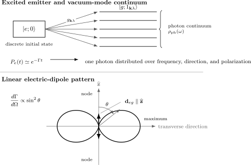
Top: a discrete excited atom–vacuum state couples to a continuum of ground-state one-photon modes; the smooth continuum produces an exponential Wigner–Weisskopf window. Bottom: a linear electric dipole has $p(\theta,\phi)\propto\sin^2\theta$, with nodes on the dipole axis.

Collection and recoil

For collection solid angle $\Omega_{\mathrm{det}}$ and polarization response $\eta(\widehat{\mathbf k},\lambda)$, the geometric collection probability is

$$\eta_{\mathrm{geom}} = \sum_\lambda \int_{\Omega_{\mathrm{det}}} d\Omega\, \eta(\widehat{\mathbf k},\lambda) p_\lambda(\widehat{\mathbf k}).$$

A scalar solid-angle fraction is insufficient when the emission pattern or detector response is anisotropic.

The mean recoil can vanish for a symmetric pattern, while the recoil variance remains nonzero. Repeated spontaneous emission therefore produces momentum diffusion even when it produces no average force by itself.

The Emitted Photon

Temporal mode

In the ideal Markov limit, after projecting onto one normalized radiative channel and suppressing its spatial and polarization label, a photon emitted from an excitation prepared at $t=0$ has temporal envelope

$$\xi(t) = \sqrt{\Gamma}\, e^{-(\Gamma/2+i\omega_c)t} \Theta(t),$$

where $\omega_c=\omega_0+\delta\omega$ is the shifted line center in this effective description. The mode is normalized because

$$\int_{-\infty}^{\infty} dt\, |\xi(t)|^2 = \int_0^\infty dt\, \Gamma e^{-\Gamma t} = 1.$$

The intensity envelope decays with the population lifetime, while the field amplitude envelope decays twice as slowly.

Spectral mode

With the Fourier convention

$$\widetilde\xi(\omega) = \frac{1}{\sqrt{2\pi}} \int_{-\infty}^{\infty} dt\, \xi(t)e^{i\omega t},$$

one obtains

$$\widetilde\xi(\omega) = \sqrt{ \frac{\Gamma}{2\pi} } \frac{1}{ \Gamma/2-i(\omega-\omega_c) }.$$

Therefore

$$|\widetilde\xi(\omega)|^2 = \frac{1}{2\pi} \frac{ \Gamma }{ (\omega-\omega_c)^2 + (\Gamma/2)^2 }.$$

The time–frequency relation is one statement about a single photon mode, not evidence that the photon possessed both an exact emission time and an exact frequency.

Detection time

Without monitoring, the atom–field state evolves coherently into a superposition of vacuum-excited and one-photon-ground components. A detector click conditions the state on one record. In a Markov photon-counting model,

$$\Pr( \text{click in }[t,t+dt] ) = \eta\Gamma \rho_{ee}(t) dt,$$

up to dark counts, collection losses, and detector response. The random click time is not a hidden classical time at which an otherwise definite photon was launched.

Which-path information

If decay can end in distinct final states,

$$|\Psi\rangle \sim \sum_f \int d\mu\, c_f(\mu) |f;1_\mu\rangle.$$

Frequency, polarization, direction, or recoil may reveal $f$. Tracing over those distinguishable photon labels suppresses coherence between final matter states. Conversely, indistinguishable decay paths can interfere. Branching fractions alone do not contain that phase information.

Relation to QED and Open Systems

Effective quantum electrodynamics

The dipole Hamiltonian is a controlled low-energy reduction of quantum electrodynamics. It quantizes the radiation field and retains the relevant matter transition, but it is not the complete relativistic theory.

Full precision work may require:

• gauge-consistent matter and field truncation;
• counter-rotating and diamagnetic terms;
• relativistic and radiative corrections to matter states;
• ultraviolet regularization and mass or frequency renormalization;
• multiphoton and higher-multipole channels;
• collective or medium-dependent electromagnetic response.

The finite decay rate is directly captured by low-energy quantum optics. The absolute Lamb shift requires more careful renormalized QED bookkeeping.

Reduced master equation

Tracing over unobserved radiation modes after the same weak-coupling and Markov steps gives

$$\dot\rho = - \frac{i}{\hbar} \left[ H_0+H_{\mathrm{LS}}, \rho \right] + \Gamma \mathcal D[\sigma_-]\rho.$$

The jump operator is

$$L = \sqrt{\Gamma}\, \sigma_-.$$

The Lindblad equation preserves the atom’s trace because the photon has been removed from the explicit state space. Its jump term repopulates the lower state, while its anticommutator terms remove excited amplitude. The Quantum Optical Master Equation derives this reduced description, and Photon Counting develops the conditioned record.

Driven atoms

For a coherently driven emitter, spontaneous emission does more than add an exponential envelope. It changes populations, damps optical coherence, produces stochastic recoil, and creates resonance fluorescence. The Optical Bloch Equations own that driven problem.

Structured Environments and the Purcell Effect

The rate is not an immutable atomic property

The transition dipole belongs to the emitter. The electromagnetic mode structure belongs to the environment. A mirror, dielectric interface, waveguide, cavity, photonic crystal, or absorbing body changes the modes sampled by the dipole and can enhance, suppress, redirect, or quench decay.

For a general linear electromagnetic environment, the weak-coupling rate can be written with the dyadic Green tensor:

$$\begin{aligned} \Gamma( \mathbf r_0,\omega_0 ) ={}& \frac{ 2\omega_0^2 }{ \hbar\epsilon_0c^2 } \\ &\times \mathbf d_{eg}^* \mathbin{\cdot} \operatorname{Im} \mathbf G( \mathbf r_0,\mathbf r_0;\omega_0 ) \mathbin{\cdot} \mathbf d_{eg}. \end{aligned}$$

This expression displays the position, frequency, and orientation dependence of the projected local density of optical states. In free space,

$$\operatorname{Im} \mathbf G_0( \mathbf r_0,\mathbf r_0;\omega ) = \frac{\omega}{6\pi c} \mathbf I,$$

which recovers the free-space E1 rate.

In absorbing structures, the Green tensor includes both radiative escape and nonradiative transfer into the material. A faster total decay rate need not mean more useful far-field photons.

Purcell-factor preview

The phrase Purcell factor denotes a rate ratio relative to a declared reference environment, but authors place either the total electromagnetic decay or one selected resonator channel in the numerator. For a total-rate definition,

$$F_P^{(\mathrm{tot})} = \frac{ \Gamma_{\mathrm{env}} }{ \Gamma_{\mathrm{ref}} }.$$

For an ideal weakly coupled emitter, optimally located and aligned with one resonant cavity mode,

$$F_P^{\mathrm{max}} = \frac{3}{4\pi^2} \left( \frac{\lambda_0}{n} \right)^3 \frac{Q}{ V_{\mathrm{eff}} }.$$

For cavity angular-frequency FWHM

$$\kappa = \frac{\omega_c}{Q},$$

a useful narrow-emitter estimate for the rate into that mode is

$$\begin{aligned} \frac{ \Gamma_{\mathrm{cav}} }{ \Gamma_{\mathrm{ref}} } \simeq \frac{ F_P^{\mathrm{max}}\mathcal O }{ 1+ 4(\omega_0-\omega_c)^2/\kappa^2 }, \end{aligned}$$

where $0\le\mathcal O\le1$ collects spatial and polarization overlap.

The equivalent bad-cavity expression is

$$\Gamma_{\mathrm{cav}} \simeq \frac{ 4g^2 }{ \kappa } \frac{1}{ 1+ 4(\omega_0-\omega_c)^2/\kappa^2 }.$$

The total population loss must still include background radiative channels and nonradiative loss:

$$\Gamma_{\mathrm{tot}} = \Gamma_{\mathrm{bg}} + \Gamma_{\mathrm{cav}} + \Gamma_{\mathrm{nr}}.$$

Where the textbook Purcell formula stops

The $Q/V_{\mathrm{eff}}$ expression is not universal. It can fail when:

• emitter and cavity are strongly coupled;
• the emitter linewidth exceeds or competes with the cavity linewidth;
• several lossy or overlapping modes contribute;
• material absorption converts energy into heat;
• the mode volume is ill-defined in an open or highly dispersive system;
• spectral diffusion or phonon sidebands dominate overlap;
• local-field corrections are important;
• collective emitters cannot be treated independently.

When coherent coupling $g$ competes with the cavity and emitter damping rates, excitation can oscillate between atom and cavity. Then normal-mode splitting or vacuum Rabi dynamics replaces a single enhanced exponential rate.

Inhibition as well as enhancement

Reducing the projected mode density can inhibit emission. Photonic band gaps, cavity detuning, polarization mismatch, or a node of the electric field can suppress a channel. In an ideal complete band gap, the continuum assumption itself fails and an atom–photon bound state can retain part of the excitation.

Purcell enhancement and inhibited emission are therefore two sides of one principle: radiative decay is a property of the coupled emitter and electromagnetic environment.

Experimental Forward Models

Time-resolved fluorescence

After an impulsive preparation, a simple detected photon-rate model is

$$R_{\mathrm{det}}(t) = \eta \Gamma_{\mathrm{rad}} P_e(0) e^{-\Gamma_{\mathrm{tot}}t} + b(t).$$

A measured histogram also contains the instrument response:

$$S(t) = \left[ h_{\mathrm{IRF}} * R_{\mathrm{det}} \right](t).$$

Fitting a bare exponential when timing jitter, a finite excitation pulse, background, detector afterpulsing, or repumping is unresolved can bias the lifetime.

Multiexponential signals

A sum of exponentials can arise from:

• several excited states;
• metastable shelving;
• different emitter orientations or environments;
• energy transfer;
• spectral diffusion;
• time-dependent quenching;
• unresolved optical pumping.

It is not automatically evidence for non-Markovian vacuum dynamics. Conversely, forcing one exponential can hide real state structure.

Separate rate, yield, and collection

Three experimentally distinct quantities are:

$$\text{lifetime} \longleftrightarrow \Gamma_{\mathrm{tot}},$$ $$\text{quantum yield} \longleftrightarrow \frac{ \Gamma_{\mathrm{rad}} }{ \Gamma_{\mathrm{tot}} },$$

and

$$\begin{gathered} \text{detected brightness} \\ \longleftrightarrow \text{preparation} \times \Phi \\ {}\times \eta_{\mathrm{geom}} \times \eta_{\mathrm{det}}. \end{gathered}$$

No one of these determines the other two without a model.

Useful cross-checks

1. Measure lifetime while varying collection optics; a true lifetime should not depend on detector solid angle.
2. Compare integrated photons with independently calibrated collection and detector efficiencies.
3. Resolve polarization and direction when magnetic sublevels matter.
4. Vary emitter–surface distance or cavity detuning to test environmental modification.
5. Compare spectral FWHM with $1/(2\pi\tau)$ to identify extra dephasing.
6. Check pump-power dependence to exclude saturation, stimulated processes, and optical pumping.
7. Fit all radiative branches with one shared upper-state lifetime.

A Reliable Calculation Workflow

1. Specify the initial and final matter states. Include magnetic, vibrational, and motional labels.
2. Choose the interaction. E1, M1, E2, two-photon, or another channel.
3. State the electromagnetic environment. Free space, homogeneous dielectric, interface, cavity, waveguide, or absorbing structure.
4. Compute matrix elements. Apply symmetry before integrating modes.
5. Build the mode coupling. Keep normalization and polarization conventions explicit.
6. Check the continuum approximation. Compare reservoir correlation, propagation, and recurrence times with the lifetime.
7. Derive partial rates. Sum only over declared final states and field channels.
8. Add nonradiative processes separately. Do not hide them inside a radiative matrix element.
9. Map to the observable. Lifetime, spectrum, angular distribution, recoil, and detected counts require different projections.
10. Test limiting cases. Recover norm conservation before tracing, free-space $\omega_0^3$ scaling, and the no-memory exponential window.

Common Mistakes

• Treating vacuum energy as a gas of real photons. The relevant statement is the nonzero field-operator matrix element between vacuum and one-photon states.
• Claiming a prescribed classical zero field causes decay. A damping term can be inserted semiclassically, but it is not derived from that zero field.
• Calling $\Gamma$ a property of the atom alone. The rate also samples the electromagnetic environment.
• Confusing amplitude and population decay. The Wigner–Weisskopf amplitude decays at $\Gamma/2$ and population at $\Gamma$.
• Dropping $2\pi$ between angular and ordinary frequency. For one lifetime-limited upper state, $\Delta\nu_{\mathrm{FWHM}}=1/(2\pi\tau)$.
• Equating observed lifetime with radiative lifetime. Nonradiative and collisional channels shorten the former.
• Assuming exact exponential decay at all times. The exact short-time survival probability is quadratic, and structured reservoirs can retain memory.
• Using a continuum rate for one lossless mode. One coherent cavity mode produces reversible exchange rather than irreversible golden-rule decay.
• Equating Purcell factor with brightness. Lossy near fields can increase total decay while decreasing radiative yield.
• Ignoring polarization and sublevel branching. Angular momentum is carried by the emitted field and the final matter state.
• Assigning a pre-existing classical emission time. A detection time is a stochastic measurement record.

Further Connections

• Einstein Coefficient Reference converts channel $A$ values into radiative lifetimes, branches, natural widths, $B$ coefficients, and oscillator strengths.
• Light Quanta to Photons gives the historical and operational route from light quanta to the modern photon concept.
• Thermal and Vacuum Noise places the $N+1$ vacuum term inside reservoir correlation functions.
• Atomic Selection Rules identifies allowed radiative branches and their angular-momentum structure.
• Fluorescence and Phosphorescence connects radiative decay to Jablonski diagrams, quantum yields, and molecular relaxation pathways.
• Line Shapes and Broadening separates natural width from Doppler, collision, transit-time, power, and instrumental effects.
• Photon Counting gives the conditioned jump statistics of detected emission.
• Cavity QED continues from Purcell-modified weak coupling to coherent strong coupling and cavity-enhanced collection.
• The open-system cavity-QED map develops conditional records, jumps, and monitored output channels.
• Transition Rates in Light–Matter Interaction supplies the detailed mode sum and occupation-factor derivation.
• Radiation Pressure uses the emitted angular distribution to separate mean optical force from recoil diffusion and heating.

References

• P. A. M. Dirac, “The Quantum Theory of the Emission and Absorption of Radiation,” Proceedings of the Royal Society A 114, 243–265 (1927), doi:10.1098/rspa.1927.0039.
• V. Weisskopf and E. Wigner, “Berechnung der natürlichen Linienbreite auf Grund der Diracschen Lichttheorie,” Zeitschrift für Physik 63, 54–73 (1930), doi:10.1007/BF01336768.
• E. M. Purcell, “Spontaneous Emission Probabilities at Radio Frequencies,” Physical Review 69, 681 (1946), doi:10.1103/PhysRev.69.681.
• D. Kleppner, “Inhibited Spontaneous Emission,” Physical Review Letters 47, 233–236 (1981), doi:10.1103/PhysRevLett.47.233.
• E. Yablonovitch, “Inhibited Spontaneous Emission in Solid-State Physics and Electronics,” Physical Review Letters 58, 2059–2062 (1987), doi:10.1103/PhysRevLett.58.2059.
• L. Fonda, G. C. Ghirardi, and A. Rimini, “Decay Theory of Unstable Quantum Systems,” Reports on Progress in Physics 41, 587–631 (1978), doi:10.1088/0034-4885/41/4/003.
• P. Lodahl, S. Mahmoodian, and S. Stobbe, “Interfacing Single Photons and Single Quantum Dots with Photonic Nanostructures,” Reviews of Modern Physics 87, 347–400 (2015), doi:10.1103/RevModPhys.87.347.
• C. Cohen-Tannoudji, J. Dupont-Roc, and G. Grynberg, Atom–Photon Interactions: Basic Processes and Applications, Wiley, 1992.
• M. O. Scully and M. S. Zubairy, Quantum Optics, Cambridge University Press, 1997.
• P. W. Milonni, The Quantum Vacuum: An Introduction to Quantum Electrodynamics, Academic Press, 1994.
• L. Novotny and B. Hecht, Principles of Nano-Optics, 2nd ed., Cambridge University Press, 2012.

Exercises

1. A zero mean field with a nonzero transition matrix element

For one mode, take

$$\mathbf E = i\mathcal E \left( \boldsymbol\epsilon a - \boldsymbol\epsilon^*a^\dagger \right).$$

1. Show that $\langle0|\mathbf E|0\rangle=0$.
2. Evaluate $\langle1|\mathbf E|0\rangle$.
3. Explain why these two results are compatible.

Solution

Because

$$a|0\rangle = 0$$

and number states with different occupation are orthogonal,

$$\langle0|a|0\rangle = \langle0|a^\dagger|0\rangle = 0.$$

Therefore

$$\langle0|\mathbf E|0\rangle = 0.$$

For the vacuum-to-one-photon matrix element,

$$\langle1|a|0\rangle = 0,$$

while

$$\langle1|a^\dagger|0\rangle = 1.$$

Hence

$$\langle1|\mathbf E|0\rangle = -i\mathcal E \boldsymbol\epsilon^*.$$

An expectation value probes the field within one state. A transition matrix element probes the coupling between two different states. A zero vacuum mean field therefore does not imply zero coupling from the vacuum to a one-photon state.

2. Derive the memory kernel

Starting from

$$\begin{aligned} \dot c_e(t) &= -i \sum_\mu g_\mu e^{i(\omega_0-\omega_\mu)t} c_\mu(t), \\ \dot c_\mu(t) &= -i g_\mu^* e^{-i(\omega_0-\omega_\mu)t} c_e(t), \end{aligned}$$

with $c_\mu(0)=0$, eliminate the field amplitudes and obtain the exact integro-differential equation for $c_e(t)$.

Solution

Integrating the second equation gives

$$c_\mu(t) = -i g_\mu^* \int_0^t d\tau\, e^{-i(\omega_0-\omega_\mu)\tau} c_e(\tau).$$

Insert this into the first equation:

$$\begin{aligned} \dot c_e(t) ={}& - \sum_\mu |g_\mu|^2 \\ &\times \int_0^t d\tau\, e^{i(\omega_0-\omega_\mu)(t-\tau)} c_e(\tau). \end{aligned}$$

Defining

$$K(s) = \sum_\mu |g_\mu|^2 e^{i(\omega_0-\omega_\mu)s}$$

gives

$$\dot c_e(t) = - \int_0^t d\tau\, K(t-\tau)c_e(\tau).$$

No irreversible or Markov approximation has yet been made. All memory is contained in $K(s)$.

3. Integrate the linear-dipole pattern

For $\mathbf d=d\widehat{\mathbf z}$, show that the differential rate

$$\frac{d\Gamma}{d\Omega} = \frac{ \omega_0^3d^2 }{ 8\pi^2\epsilon_0\hbar c^3 } \sin^2\theta$$

integrates to the standard free-space rate.

Solution

The angular integral is

$$\begin{aligned} \int d\Omega\, \sin^2\theta &= 2\pi \int_0^\pi d\theta\, \sin^3\theta \\ &= \frac{8\pi}{3}. \end{aligned}$$

Therefore

$$\begin{aligned} \Gamma &= \frac{ \omega_0^3d^2 }{ 8\pi^2\epsilon_0\hbar c^3 } \frac{8\pi}{3} \\ &= \frac{ \omega_0^3d^2 }{ 3\pi\epsilon_0\hbar c^3 }. \end{aligned}$$

The corresponding normalized angular distribution is

$$p(\theta,\phi) = \frac{3}{8\pi} \sin^2\theta.$$

4. Lifetime and natural linewidth

An excited state has a lifetime

$$\tau = 26.0\ \mathrm{ns}.$$

Assume the lower state is stable and there is no pure dephasing. Find:

1. the population-decay rate $\Gamma$;
2. the angular-frequency FWHM;
3. the ordinary-frequency FWHM.

Solution

The population rate is

$$\begin{aligned} \Gamma &= \frac{1}{\tau} \\ &= \frac{1}{ 26.0\times10^{-9}\ \mathrm s } \\ &\simeq 3.85\times10^7\ \mathrm{s^{-1}}. \end{aligned}$$

For the stated lifetime-limited transition,

$$\Delta\omega_{\mathrm{FWHM}} = \Gamma \simeq 3.85\times10^7\ \mathrm{rad\,s^{-1}}.$$

The ordinary-frequency width is

$$\begin{aligned} \Delta\nu_{\mathrm{FWHM}} &= \frac{\Gamma}{2\pi} \\ &\simeq 6.12\ \mathrm{MHz}. \end{aligned}$$

5. Branching and quantum yield

An excited state has radiative rates

$$\Gamma_1 = 2.0\times10^7\ \mathrm{s^{-1}},$$ $$\Gamma_2 = 1.0\times10^7\ \mathrm{s^{-1}},$$

and a nonradiative rate

$$\Gamma_{\mathrm{nr}} = 0.5\times10^7\ \mathrm{s^{-1}}.$$

Find the observed lifetime, radiative quantum yield, radiative branching fractions, and the probability per preparation of producing a photon in channel 1.

Solution

The total rate is

$$\begin{aligned} \Gamma_{\mathrm{tot}} &= \Gamma_1+\Gamma_2+\Gamma_{\mathrm{nr}} \\ &= 3.5\times10^7\ \mathrm{s^{-1}}. \end{aligned}$$

Thus

$$\tau_{\mathrm{obs}} = \frac{1}{\Gamma_{\mathrm{tot}}} \simeq 28.6\ \mathrm{ns}.$$

The total radiative rate is

$$\Gamma_{\mathrm{rad}} = 3.0\times10^7\ \mathrm{s^{-1}},$$

so

$$\Phi = \frac{\Gamma_{\mathrm{rad}}}{ \Gamma_{\mathrm{tot}} } = \frac{6}{7} \simeq 0.857.$$

The radiative branching fractions are

$$b_1^{(\mathrm{rad})} = \frac23, \qquad b_2^{(\mathrm{rad})} = \frac13.$$

The probability per preparation of emitting through channel 1 is instead

$$\frac{\Gamma_1}{ \Gamma_{\mathrm{tot}} } = \frac47 \simeq 0.571.$$

It includes competition with the nonradiative channel and is therefore not equal to the radiative branching fraction.

6. Normalize the emitted photon

For

$$\xi(t) = \sqrt{\Gamma}\, e^{-(\Gamma/2+i\omega_c)t} \Theta(t),$$

show that the temporal mode is normalized and that its spectral probability has angular FWHM $\Gamma$.

Solution

The temporal norm is

$$\begin{aligned} \int_{-\infty}^{\infty} dt\, |\xi(t)|^2 &= \int_0^\infty dt\, \Gamma e^{-\Gamma t} \\ &= 1. \end{aligned}$$

The Fourier transform is

$$\widetilde\xi(\omega) = \sqrt{ \frac{\Gamma}{2\pi} } \frac{1}{ \Gamma/2-i(\omega-\omega_c) }.$$

Hence

$$|\widetilde\xi(\omega)|^2 = \frac{1}{2\pi} \frac{\Gamma}{ (\omega-\omega_c)^2+(\Gamma/2)^2 }.$$

At half maximum,

$$|\omega-\omega_c| = \frac{\Gamma}{2}.$$

The separation between the two half-maximum points is therefore

$$\Delta\omega_{\mathrm{FWHM}} = \Gamma.$$

7. Why exact decay starts quadratically

Let

$$A(t) = \langle\psi| e^{-iHt/\hbar} |\psi\rangle.$$

Expand to second order in $t$ and show that

$$|A(t)|^2 = 1 - \frac{ (\Delta H)^2 }{ \hbar^2 } t^2 + o(t^2).$$

Why does this rule out an exact exponential at arbitrarily short times?

Solution

Expanding the evolution operator,

$$\begin{aligned} A(t) ={}& 1 - \frac{i}{\hbar} \langle H\rangle t \\ &\quad - \frac{1}{2\hbar^2} \langle H^2\rangle t^2 + o(t^2). \end{aligned}$$

Multiplying by the complex conjugate gives

$$\begin{aligned} |A(t)|^2 &= 1 - \frac{ \langle H^2\rangle - \langle H\rangle^2 }{ \hbar^2 } t^2 + o(t^2) \\ &= 1 - \frac{ (\Delta H)^2 }{ \hbar^2 } t^2 + o(t^2). \end{aligned}$$

The initial derivative is zero. By contrast,

$$e^{-\Gamma t} = 1-\Gamma t+O(t^2)$$

has a nonzero negative initial derivative. Exponential decay is therefore an intermediate-time approximation, not an exact law from $t=0$.

8. A cavity Purcell estimate

An ideal cavity has

$$Q = 10^4, \qquad V_{\mathrm{eff}} = 2 \left( \frac{\lambda_0}{n} \right)^3.$$

The emitter has overlap $\mathcal O=0.25$ and detuning

$$|\omega_0-\omega_c| = \frac{\kappa}{2}.$$

1. Estimate $F_P^{\mathrm{max}}$.
2. Estimate $\Gamma_{\mathrm{cav}}/\Gamma_{\mathrm{ref}}$.
3. If the unmodified background remains $\Gamma_{\mathrm{ref}}$ and there is no nonradiative loss, estimate the fraction of emission entering the cavity channel.

Solution

The ideal maximum factor is

$$\begin{aligned} F_P^{\mathrm{max}} &= \frac{3}{4\pi^2} \frac{Q}{2} \\ &\simeq 3.80\times10^2. \end{aligned}$$

The overlap contributes $0.25$. At $|\omega_0-\omega_c|=\kappa/2$, the Lorentzian denominator is

$$1+ 4 \frac{ (\kappa/2)^2 }{ \kappa^2 } = 2.$$

Therefore

$$\frac{ \Gamma_{\mathrm{cav}} }{ \Gamma_{\mathrm{ref}} } \simeq \frac{ (3.80\times10^2)(0.25) }{2} \simeq 47.5.$$

With an unchanged background channel,

$$\Gamma_{\mathrm{tot}} \simeq \left( 1+47.5 \right) \Gamma_{\mathrm{ref}}.$$

The cavity-channel fraction is

$$\beta_{\mathrm{cav}} = \frac{47.5}{ 1+47.5 } \simeq 0.979.$$

This estimate assumes weak coupling, one well-defined cavity mode, a narrow emitter, and no absorptive or other nonradiative channel. A large numerical $Q/V$ value alone does not establish those assumptions.