Line Shapes and Broadening

An ideal transition has a definite frequency

$$\omega_0 = \frac{E_u-E_l}{\hbar},$$

but a measured spectral line has a center, area, width, shape, and wing structure. These features answer different physical questions. The area can track transition strength and population; the width can encode coherence loss, motion, collisions, drive strength, static disorder, or instrumental resolution; the wings can distinguish models that look nearly identical at the peak.

Write an isolated line schematically as

$$\begin{aligned} S(\omega) &= \mathcal A L(\omega-\omega_c), \\ \int_{-\infty}^{\infty} L(\delta\omega)\,d\delta\omega &=1. \end{aligned}$$

Here $\mathcal A$ is the integrated area on an angular-frequency axis and $L$ is a normalized profile. Broadening can lower the peak while leaving $\mathcal A$ unchanged. Conversely, a process that changes populations or oscillator strength can change the area as well as the shape.

The central lesson is that a linewidth is not a mechanism. It is a fitted or derived parameter whose physical meaning depends on the profile, coordinate, preparation, propagation model, and instrument.

Canonical Scope

This page owns the spectroscopy-facing derivation and use of natural, lifetime, Doppler, collisional, power, and inhomogeneous broadening. It also owns the Lorentzian-Gaussian-Voigt dictionary, the separation of intrinsic and instrumental widths, and the fitting cautions needed to extract physical parameters from measured lines.

Nearby pages retain narrower responsibilities:

• Spectroscopy gives the chapter-level measurement map and a compact profile preview.
• Transition Rates owns the rate approximation and the first lifetime-linewidth bridge.
• Absorption and Emission owns optical depth, emissivity, and radiative transfer.
• Optical Bloch Equations owns the AMO saturation curve, power-broadened width, scattering rate, and experimental forward models.
• The open-system treatment owns the general driven two-level master-equation derivation.
• Pure-Dephasing Master Equation owns Markovian phase damping and its microscopic interpretations.
• Spectral Functions owns many-body poles, continua, self-energies, and artificial numerical broadening.

This article treats mostly isolated lines. Overlapping resonances, interference profiles, line mixing, thresholds, and strongly non-Markovian dynamics can require a matrix response or a more specialized theory.

Convention Ledger

The page uses:

• $\delta\omega=\omega-\omega_c$ for angular-frequency detuning;
• $\gamma_{\mathrm L}$ for a Lorentzian half width at half maximum;
• $\sigma_{\mathrm G}$ for a Gaussian standard deviation;
• $\Gamma_1$ for a population-decay rate;
• $\Gamma_2$ for a coherence-decay rate;
• $T_1=1/\Gamma_1$ and $T_2=1/\Gamma_2$;
• $w_{\mathrm L}=2\gamma_{\mathrm L}$ for Lorentzian FWHM;
• $w_{\mathrm G}=2\sqrt{2\ln2}\,\sigma_{\mathrm G}$ for Gaussian FWHM; and
• $R(\omega)$ for a normalized instrumental response.

Rates such as $\Gamma_1$ have units of inverse seconds. When they set an angular-frequency width, the numerical unit is $\mathrm{rad\,s^{-1}}$, with radians dimensionless. Convert to ordinary-frequency width using

$$\Delta\nu = \frac{\Delta\omega}{2\pi}.$$

An energy width is

$$\Delta E = \hbar\Delta\omega = h\Delta\nu.$$

The symbol $\Gamma$ is used elsewhere for a decay rate, an angular-frequency HWHM, an angular-frequency FWHM, or an energy width. Never compare quoted values until the units and width convention are explicit.

Anatomy of a Spectral Line

Center, area, width, and shape

For a normalized line $L(\delta\omega)$:

• the center estimates a transition frequency after shifts are modeled;
• the area carries integrated spectral weight;
• the width specifies a scale only after naming HWHM, FWHM, standard deviation, or another convention;
• the shape describes the core, symmetry, and tails; and
• the wings can dominate weak neighboring features and radiative-transfer errors even when the line center fits well.

The peak value is not independent. At fixed area, a normalized Lorentzian has

$$L_{\mathrm L}(0) = \frac{1}{\pi\gamma_{\mathrm L}},$$

whereas a normalized Gaussian has

$$L_{\mathrm G}(0) = \frac{1} {\sigma_{\mathrm G}\sqrt{2\pi}}.$$

A narrower line is therefore taller at fixed area.

Homogeneous and inhomogeneous broadening

Homogeneous broadening gives every member of the selected ensemble the same dynamical profile. Markovian lifetime decay, pure dephasing, and impact- limit collisions are standard examples. A narrow subensemble does not remove the width.

Inhomogeneous broadening averages over members with different static or slowly varying centers. Thermal Doppler broadening, unresolved site shifts, and shot-to-shot detuning disorder are examples. Selecting a narrower class or refocusing slow offsets can reduce the width.

The distinction is operational. Spectral diffusion that is static during one measurement but changes between scans looks inhomogeneous; the same noise can look like homogeneous dephasing when it fluctuates rapidly during each coherence interval.

Convolution is not universal

If two statistically independent, shift-invariant broadening stages act sequentially, their profiles convolve:

$$L_{12}(\omega) = \int_{-\infty}^{\infty} L_1(\omega-\omega') L_2(\omega')\,d\omega'.$$

Static distributions also produce a convolution when the homogeneous shape does not depend on the shifted center. Correlated mechanisms, state-dependent widths, line mixing, nonlinear propagation, and saturation generally require a joint model rather than a blind convolution.

Natural Linewidth

Radiative survival

An excited level $u$ with radiative branches $u\rightarrow l$ has total radiative population-decay rate

$$\Gamma_u^{\mathrm{rad}} = \sum_l A_{ul}.$$

If this is the only loss, its population decays as

$$P_u(t) = P_u(0)e^{-\Gamma_u^{\mathrm{rad}}t}.$$

The state amplitude decays at half that rate. For a stable lower state and no additional dephasing, the transition has Lorentzian angular-frequency FWHM

$$w_{\mathrm{nat}} = \Gamma_u^{\mathrm{rad}},$$

ordinary-frequency FWHM

$$\Delta\nu_{\mathrm{nat}} = \frac{\Gamma_u^{\mathrm{rad}}}{2\pi},$$

and energy FWHM

$$\Delta E_{\mathrm{nat}} = \hbar\Gamma_u^{\mathrm{rad}}.$$

This is the natural radiative width in the simplest free-space Markov model. It is not necessarily the observed width.

Both levels can be unstable

Let the upper and lower levels lose population at rates $\Gamma_u$ and $\Gamma_l$, and let $\gamma_\phi$ be additional pure dephasing of the optical coherence. Under independent Markovian decay,

$$\Gamma_2 = \frac{\Gamma_u+\Gamma_l}{2} + \gamma_\phi.$$

The Lorentzian profile has

$$\begin{aligned} \gamma_{\mathrm L} &= \Gamma_2, \\ w_{\mathrm L} &= 2\Gamma_2 = \Gamma_u+\Gamma_l+2\gamma_\phi. \end{aligned}$$

The transition width contains the sum of level decay contributions. Using only the upper lifetime is justified only when the lower level is stable and pure dephasing is negligible.

Natural does not mean immutable

The radiative rate depends on the electromagnetic mode density. Cavities, interfaces, photonic crystals, and strong coupling can modify decay or split the response. Nonradiative loss adds lifetime broadening, while structured reservoirs can produce nonexponential decay and non-Lorentzian spectra.

Accordingly, “natural linewidth” should name the environment and model. A free-space Einstein $A$ coefficient is not a universal property of the bare matter Hamiltonian independent of its radiation field.

Lifetime Broadening

Exponential coherence gives a Lorentzian

Suppose a transition coherence for $t\ge0$ behaves as

$$C(t) = C(0) e^{-\Gamma_2t} e^{-i\omega_ct}.$$

Its one-sided Fourier response contains

$$\int_0^\infty e^{-\Gamma_2t} e^{i\delta\omega t} \,dt = \frac{1} {\Gamma_2-i\delta\omega}.$$

The absorptive part, or the squared amplitude under the matching emission model, has a Lorentzian denominator:

$$L_{\mathrm L}(\delta\omega) = \frac{1}{\pi} \frac{\Gamma_2} {\delta\omega^2+\Gamma_2^2}.$$

Thus $T_2$ sets the angular-frequency HWHM,

$$\gamma_{\mathrm L} = \frac{1}{T_2}, \qquad w_{\mathrm L} = \frac{2}{T_2}.$$

For a stable lower state with population lifetime $T_1$ and pure-dephasing time $T_\phi$,

$$\frac{1}{T_2} = \frac{1}{2T_1} + \frac{1}{T_\phi}.$$

No pure dephasing gives $T_2=2T_1$ and $w_{\mathrm L}=1/T_1$.

Total lifetime versus radiative lifetime

An upper population can disappear through radiative decay, quenching, predissociation, autoionization, chemical reaction, or escape:

$$\Gamma_u^{\mathrm{tot}} = \Gamma_u^{\mathrm{rad}} + \Gamma_u^{\mathrm{nr}}.$$

All irreversible loss from the selected upper state contributes to its survival amplitude in the stated model. Only the radiative branches produce the photons assigned to fluorescence. A broadened line and a reduced quantum yield can therefore have the same nonradiative origin.

Limits of the lifetime-width dictionary

The reciprocal relation assumes an exponential over the time interval that controls the line. It can fail or become approximate for:

• short-time quadratic survival;
• long-time nonexponential tails;
• coherent recurrences in a discrete spectrum;
• strong coupling and resolved dressed states;
• thresholds and energy-dependent continua;
• non-Markovian spectral diffusion; and
• several unresolved transitions with different centers.

Finite observation time and transit time can also broaden a line, but they do not necessarily define an intrinsic excited-state lifetime.

Doppler Broadening

Velocity-dependent resonance

For a wave propagating along $z$, a nonrelativistic absorber with velocity $v_z$ sees a first-order Doppler shift

$$\delta\omega \simeq -k_0v_z, \qquad k_0 = \frac{\omega_0}{c}.$$

For a thermal gas, one velocity component follows

$$p(v_z) = \sqrt{ \frac{m}{2\pi k_{\mathrm B}T} } \exp\!\left( -\frac{mv_z^2} {2k_{\mathrm B}T} \right).$$

Mapping velocity to detuning produces a Gaussian line with standard deviation

$$\sigma_{\mathrm D} = \frac{\omega_0}{c} \sqrt{ \frac{k_{\mathrm B}T}{m} }.$$

Its angular-frequency FWHM is

$$w_{\mathrm D} = 2\sqrt{2\ln2}\, \frac{\omega_0}{c} \sqrt{ \frac{k_{\mathrm B}T}{m} },$$

or, in fractional form,

$$\frac{\Delta\nu_{\mathrm D}} {\nu_0} = \sqrt{ \frac{8k_{\mathrm B}T\ln2} {mc^2} }.$$

The fractional first-order Doppler FWHM is the same on frequency and angular- frequency axes. A wavelength-domain profile is only approximately Gaussian for a narrow line because the frequency-wavelength map is nonlinear.

What temperature is measured?

The formula measures the velocity variance along the optical wavevector. It returns a translational temperature only for a Maxwellian distribution. Atomic beams, expanding gases, trapped particles, plasmas with unequal ion and electron temperatures, and laser-cooled clouds can be nonthermal or anisotropic.

A fitted Gaussian width can also contain laser jitter, unresolved isotope structure, static fields, or instrumental resolution. Calling every Gaussian width a Doppler temperature is therefore unsafe.

Doppler-free does not mean width-free

Counterpropagating-beam methods, saturated absorption, two-photon geometries, and trapped-particle spectroscopy can suppress first-order Doppler broadening. Natural width, transit time, recoil, collisions, laser frequency noise, power broadening, and second-order Doppler shifts can remain.

Collisional Broadening

Random phase interruptions

In the impact approximation, many short, statistically independent collisions interrupt the optical phase. A simple coherence model is

$$\begin{aligned} C(t) &\propto \exp\!\left[- (\Gamma_2^{(0)}+\gamma_{\mathrm{col}})t \right] \\ &\quad\times \exp\!\left[-i (\omega_0+\Delta_{\mathrm{col}})t \right]. \end{aligned}$$

The collision-induced HWHM $\gamma_{\mathrm{col}}$ adds to other homogeneous Lorentzian HWHMs, while $\Delta_{\mathrm{col}}$ shifts the center. At low perturber density,

$$\gamma_{\mathrm{col}} \sim n_{\mathrm p} \left\langle v_{\mathrm{rel}} \sigma_{\mathrm{broad}} \right\rangle.$$

The broadening cross section is a phase-changing collision quantity, not generally the same as an elastic or momentum-transfer cross section.

Pressure and temperature scaling

Molecular databases often tabulate a Lorentzian HWHM at reference pressure and temperature. A common empirical form is

$$\gamma_{\mathrm L}(p,T) = \left( \frac{T_{\mathrm{ref}}}{T} \right)^n \left[ \gamma_{\mathrm{air}}p_{\mathrm{air}} + \gamma_{\mathrm{self}}p_{\mathrm{self}} \right],$$

with pressure units matched to the tabulated coefficients. A pressure shift is parameterized separately. The exponent $n$ is line- and perturber- dependent; it is not a universal kinetic-theory constant.

Different collision regimes

“Pressure broadening” covers several mechanisms:

• resonance or self-broadening between identical radiators;
• van der Waals broadening by neutral perturbers;
• Stark broadening by charged particles and fluctuating electric fields;
• state-changing and quenching collisions;
• velocity-changing collisions; and
• line mixing among coupled transitions.

Impact-limit cores are often approximately Lorentzian. Quasistatic fields can produce non-Lorentzian wings, asymmetry, and density scalings that differ from the simple linear-pressure picture.

Dicke narrowing and speed dependence

Collisions do not only broaden. Frequent velocity-changing collisions can confine the phase-accumulating motion and narrow the Doppler contribution, an effect commonly called Dicke narrowing. Collisional width and shift can also depend on molecular speed.

The ordinary Voigt model omits these effects. High-resolution gas spectra can require speed-dependent profiles, hard- or soft-collision narrowing models, correlations between velocity- and state-changing collisions, and line mixing.

Power Broadening

Driven two-level result

Consider a Markovian two-level system driven with Rabi frequency $\Omega$ and detuning $\Delta$. Let $\Gamma_1$ be population decay and $\Gamma_2$ coherence decay. The steady excited-state population is

$$\rho_{ee}^{\mathrm{ss}} = \frac{ \Omega^2\Gamma_2 }{ 2\left[ \Gamma_1 (\Delta^2+\Gamma_2^2) + \Omega^2\Gamma_2 \right] }.$$

As a function of detuning, the denominator contains

$$\Delta^2 + \Gamma_2^2 \left(1+s_0\right), \qquad s_0 = \frac{\Omega^2} {\Gamma_1\Gamma_2}.$$

The ideal two-level Lorentzian HWHM is therefore

$$\gamma_{\mathrm{pow}} = \Gamma_2 \sqrt{1+s_0},$$

and the FWHM is

$$w_{\mathrm{pow}} = 2\Gamma_2 \sqrt{1+s_0}.$$

At weak drive, $s_0\ll1$, the width tends to $2\Gamma_2$. Stronger drive flattens the population response and broadens its detuning dependence.

Convention check

If pure dephasing is absent, $\Gamma_2=\Gamma_1/2$, so

$$s_0 = \frac{2\Omega^2} {\Gamma_1^2}.$$

Some authors define the Rabi frequency or saturation parameter with different factors of two. The invariant procedure is to derive the line from the stated Hamiltonian and master equation, then read off the half-maximum detuning.

When broadening becomes structure

Power broadening is not an intrinsic property of the unilluminated transition. It depends on local intensity, polarization, detuning convention, and level structure. In multilevel systems, strong light can also cause optical pumping, AC Stark shifts, Autler–Townes splitting, coherent dark states, and spatially varying saturation.

Once resolved dressed-state peaks or coherent Rabi dynamics appear, one broad Lorentzian is no longer the right description.

Inhomogeneous Broadening

Static distribution of centers

Let each microscopic member have homogeneous profile $L_{\mathrm{hom}}(\omega-\Omega)$ but a center $\Omega$ drawn from $p(\Omega)$. The ensemble profile is

$$L_{\mathrm{ens}}(\omega) = \int_{-\infty}^{\infty} p(\Omega) L_{\mathrm{hom}}(\omega-\Omega) \,d\Omega.$$

If $p$ is Gaussian and $L_{\mathrm{hom}}$ is Lorentzian, the result is a Voigt profile. If both are Gaussian, their variances add.

Sources of static or slow center variation include:

• Doppler shifts;
• isotope or unresolved hyperfine structure;
• strain, site, solvent, or local-field distributions;
• spatially varying Zeeman, Stark, or trapping fields;
• laser-frequency drift between shots; and
• slow spectral diffusion.

Unresolved structure is sometimes called broadening, but it can be a sum of several sharp lines rather than one broadened transition.

T2 star and refocusing

Quasi-static detuning noise causes ensemble coherence to decay on a time $T_2^*$ that can be much shorter than the homogeneous $T_2$. A spin echo or photon echo can refocus sufficiently slow, reversible offsets, revealing a longer coherence time.

An echo cannot undo population loss, fast Markovian dephasing, or every form of spectral diffusion. The difference between $T_2^*$ and $T_2$ is a useful diagnostic, not a universal partition into Gaussian and Lorentzian widths.

Spatial selection and hole burning

An inhomogeneous ensemble can contain narrow spectral classes. State selection, spectral hole burning, or sufficiently narrow excitation can probe a subset whose width is closer to the homogeneous line. The measured hole still includes pump power, population dynamics, diffusion, and probe resolution.

Lorentzian, Gaussian, and Voigt Profiles

Lorentzian

The normalized Lorentzian is

$$L_{\mathrm L} (\delta\omega;\gamma_{\mathrm L}) = \frac{1}{\pi} \frac{\gamma_{\mathrm L}} {\delta\omega^2+\gamma_{\mathrm L}^2}.$$

It has HWHM $\gamma_{\mathrm L}$, FWHM $w_{\mathrm L}=2\gamma_{\mathrm L}$, and algebraic wings $L_{\mathrm L}\sim\delta\omega^{-2}$. Its ordinary variance does not exist on an infinite domain.

Lorentzians arise from ideal exponential coherence, impact-limit phase interruptions, and isolated weakly damped poles. They should not be assigned automatically to every broadened peak.

Gaussian

The normalized Gaussian is

$$L_{\mathrm G} (\delta\omega;\sigma_{\mathrm G}) = \frac{1} {\sigma_{\mathrm G}\sqrt{2\pi}} \exp\!\left[ -\frac{\delta\omega^2} {2\sigma_{\mathrm G}^2} \right].$$

Its FWHM is

$$w_{\mathrm G} = 2\sqrt{2\ln2}\, \sigma_{\mathrm G}.$$

Gaussians arise from normal distributions of shifts and from several independent Gaussian resolution sources. Their tails fall much faster than Lorentzian wings.

Voigt

The Voigt profile is the convolution

$$\begin{aligned} L_{\mathrm V} (\delta\omega;\sigma_{\mathrm G},\gamma_{\mathrm L}) &= \int_{-\infty}^{\infty} L_{\mathrm G}(x;\sigma_{\mathrm G}) \\ &\quad\times L_{\mathrm L} (\delta\omega-x;\gamma_{\mathrm L}) \,dx. \end{aligned}$$

Using the Faddeeva function

$$w(z) = e^{-z^2} \operatorname{erfc}(-iz),$$

one may write

$$L_{\mathrm V} = \frac{\operatorname{Re}w(z)} {\sigma_{\mathrm G}\sqrt{2\pi}}, \qquad z = \frac{\delta\omega+i\gamma_{\mathrm L}} {\sigma_{\mathrm G}\sqrt2}.$$

The Voigt profile is normalized. Its core can be Gaussian-dominated, but any nonzero Lorentzian component controls the far-wing asymptote.

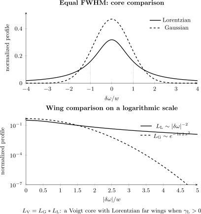
Normalized Lorentzian and Gaussian profiles with the same FWHM can look similar near half maximum while differing strongly in peak height and wings. A Voigt convolution inherits Lorentzian far wings whenever $\gamma_{\mathrm L}>0$.

Combining widths

Two Lorentzian convolutions add HWHMs:

$$\gamma_{\mathrm L,tot} = \gamma_{\mathrm L,1} + \gamma_{\mathrm L,2}.$$

Two Gaussian convolutions add variances:

$$\sigma_{\mathrm G,tot}^2 = \sigma_{\mathrm G,1}^2 + \sigma_{\mathrm G,2}^2.$$

Therefore Gaussian FWHMs add in quadrature, not linearly. A Gaussian and a Lorentzian form a Voigt profile, whose FWHM has no elementary exact formula. A useful approximation is

$$w_{\mathrm V} \simeq 0.5346w_{\mathrm L} + \sqrt{ 0.2166w_{\mathrm L}^2 + w_{\mathrm G}^2 }.$$

This estimates the total FWHM; it does not separate mechanisms from one measured number.

When Voigt is not enough

The Voigt profile assumes a Gaussian distribution of Doppler shifts convolved with a velocity-independent Lorentzian collision width and shift. Precision gas spectroscopy can resolve omitted physics such as speed-dependent collisions, velocity-changing collisions, Dicke narrowing, correlations, and line mixing.

An IUPAC task group recommended the Hartmann-Tran profile in 2014 as a beyond-Voigt isolated-line model. The current HITRAN2024 framework, published in 2026, recommends a modified Hartmann-Tran profile for cases in which beyond-Voigt effects matter. This mHT representation uses a quadratic speed-dependent hard-collision profile with double-power-law temperature dependences and replaces HITRAN’s earlier preferred HT parameterization.

This is a database and high-resolution modeling recommendation, not a claim that every spectrum needs the most elaborate profile. The simplest model that leaves statistically and physically acceptable residuals is often the most identifiable.

Instrumental and Finite-Time Broadening

Instrument response

A spectrometer records a response-convolved signal:

$$S_{\mathrm{meas}}(\omega) = \int_{-\infty}^{\infty} R(\omega-\omega') S_{\mathrm{true}}(\omega') \,d\omega',$$

with

$$\int R(\omega)\,d\omega =1$$

when the apparatus function preserves area. Slit functions, diffraction, detector pixels, interferometer windows, laser linewidth, and frequency noise can all contribute.

Resolving power is commonly quoted as

$$\mathcal R = \frac{\nu}{\Delta\nu},$$

but $\Delta\nu$ must still be tied to an instrument-profile convention. Two features separated by one quoted FWHM are not automatically resolved under every criterion.

Finite observation and pulse duration

A rectangular observation of duration $T$ produces a sinc-like amplitude window and sinc-squared intensity response. A Gaussian pulse produces a Gaussian transform-limited envelope. Apodization changes sidelobes and width.

This Fourier width is a property of preparation or observation. It should not be added to a lifetime rate unless the full temporal model shows that the corresponding kernels convolve or decay rates add.

Laser frequency noise

Fast white frequency noise can resemble homogeneous dephasing. Slow drift can produce an inhomogeneous distribution between scans. Intermediate colored noise produces profile shapes that depend on acquisition time and scan protocol. Quoting only the laser’s nominal linewidth can be insufficient.

Deconvolution and Fitting Cautions

Fit a forward model

For sampled data $y_k$, a defensible model has the form

$$y_k = \left[ R*S_{\mathrm{phys}} \right](\omega_k) + b(\omega_k) + \epsilon_k,$$

where $S_{\mathrm{phys}}$ contains all resolved lines, $R$ is the calibrated instrument response, $b$ is a baseline or background, and $\epsilon_k$ is a noise model.

Fit this forward-convolved model to the data. Deconvolving first and fitting later usually creates correlated noise and unstable artifacts.

Why direct deconvolution is ill conditioned

In Fourier space,

$$\widetilde S_{\mathrm{meas}}(t) = \widetilde R(t) \widetilde S_{\mathrm{true}}(t).$$

Formal inversion divides by $\widetilde R(t)$. Where the transfer function is small, noise is amplified:

$$\widetilde S_{\mathrm{true}}(t) = \frac{ \widetilde S_{\mathrm{meas}}(t) }{ \widetilde R(t) }.$$

Regularization imposes prior smoothness or sparsity and therefore changes the estimator. A deconvolved line should be reported with the regularization, resolution, uncertainty, and validation tests.

Model hierarchy

A useful progression is:

1. calibrate the frequency axis and instrumental response;
2. fit a physically justified Lorentzian or Gaussian limit;
3. fit a Voigt profile if independent Gaussian and Lorentzian mechanisms are plausible;
4. add neighboring lines, asymmetry, or pressure shifts when residuals demand them;
5. use speed-dependent, narrowing, line-mixing, or mHT models only with data capable of constraining the added parameters; and
6. compare residual structure, parameter stability, and predictive behavior across pressures, powers, or temperatures.

More parameters always reduce an unconstrained least-squares residual. They do not automatically improve the physical inference.

Baselines, overlap, and finite windows

Line wings can trade off strongly against polynomial baselines and neighboring features. A fit window that is too narrow cannot determine Lorentzian tails; a window that is too broad may require a more realistic continuum model.

Integrated area is conserved by a normalized convolution only on the full axis. Finite windows, clipped detector ranges, variable throughput, and nonlinear transmittance can spoil apparent area conservation.

Coordinate transformations

Profiles are densities. Under

$$\omega = \frac{2\pi c}{\lambda},$$

one must transform

$$L_\lambda(\lambda) = L_\omega(\omega) \frac{2\pi c}{\lambda^2}.$$

A symmetric line in frequency is not exactly symmetric in wavelength. Fit in the coordinate for which the physical and instrumental model is defined, then transform the final density with its Jacobian.

Worked Example: Natural and Doppler Widths

Consider an optical transition at

$$\lambda_0 = 500\ \mathrm{nm}$$

in an atom of mass $m=40\,u$ at $T=300\ \mathrm K$. Let the upper population lifetime be $T_1=10\ \mathrm{ns}$, with a stable lower level and no pure dephasing.

The ordinary-frequency natural FWHM is

$$\Delta\nu_{\mathrm{nat}} = \frac{1}{2\pi T_1} \simeq 15.9\ \mathrm{MHz}.$$

The line frequency is

$$\nu_0 = \frac{c}{\lambda_0} \simeq 5.996\times10^{14}\ \mathrm{Hz}.$$

The Doppler FWHM is

$$\Delta\nu_{\mathrm D} = \nu_0 \sqrt{ \frac{8k_{\mathrm B}T\ln2} {mc^2} } \simeq 1.18\ \mathrm{GHz}.$$

The Doppler core is roughly $74$ times wider than the natural FWHM. Using the Voigt approximation with

$$w_{\mathrm L}=15.9\ \mathrm{MHz}, \qquad w_{\mathrm G}=1.18\ \mathrm{GHz},$$

gives

$$w_{\mathrm V} \simeq 1.19\ \mathrm{GHz}.$$

The FWHM is almost Doppler limited, yet the natural Lorentzian component still controls sufficiently remote wings. A Gaussian-only fit can therefore recover the core width while underpredicting wing absorption.

Practical Workflow

1. Name the spectral coordinate. Frequency, angular frequency, wavenumber, wavelength, and energy densities require Jacobians.
2. Separate center, area, and width. Do not use peak height as a proxy for all three.
3. Declare width conventions. Record HWHM, FWHM, standard deviation, and whether the number is angular frequency, hertz, or energy.
4. List candidate mechanisms. Include lifetimes, dephasing, motion, collisions, drive, static distributions, transit time, and apparatus.
5. Estimate scales before fitting. Compare expected natural, Doppler, pressure, power, and resolution widths.
6. Use a forward model. Convolve the physical spectrum with a calibrated response and include baseline and neighboring lines.
7. Vary control parameters. Pressure, temperature, power, beam geometry, and observation time help separate mechanisms.
8. Inspect residuals and covariance. Structured residuals reveal model failure; strong covariance reveals weak identifiability.
9. Test fit-window stability. Centers, areas, and widths should not drift without physical explanation.
10. Report provenance. State whether widths were observed, fitted, calculated, deconvolved, or taken from a database.

Common Mistakes

Writing linewidth equals inverse lifetime without conventions

The relation depends on whether the lifetime describes population or coherence and whether the width is HWHM, FWHM, angular frequency, ordinary frequency, or energy.

Treating natural and observed widths as identical

Doppler motion, collisions, drive, static disorder, unresolved structure, laser noise, and instrument response can all dominate the radiative width.

Adding every FWHM linearly

Lorentzian HWHMs add under convolution. Gaussian variances add. Voigt and more general profiles require their own forward calculation.

Calling every Gaussian width Doppler broadening

Static fields, isotope mixtures, laser jitter, and Gaussian instrument functions can produce the same elementary shape.

Calling every Lorentzian width a lifetime

Impact collisions, laser phase diffusion, a chosen numerical regulator, and some instrument functions can be Lorentzian without measuring the target’s population lifetime.

Treating power broadening as a material constant

It depends on local Rabi frequency and relaxation. Spatial intensity variation can itself make the ensemble profile non-Lorentzian.

Assuming a Voigt fit proves two mechanisms

A Voigt curve can be an effective fit to unresolved structure or other physics. Parameter plausibility and control-variable scaling are needed.

Interpreting unresolved splitting as one decay width

Several narrow transitions can mimic one broad line. Better resolution, field dependence, polarization, or a constrained multiplet model may reveal the components.

Deconvolving by subtracting widths

Linear subtraction works only for Lorentzian FWHMs under the matching convolution model. Gaussian widths subtract in quadrature. A Voigt instrument requires a Voigt-aware fit.

Ignoring line shifts while fitting widths

Collisions, AC Stark effects, recoil, and calibration errors can move the center. Width and shift parameters can be correlated.

Trusting a small fit error under a wrong profile

Statistical covariance assumes the model family is adequate. It does not include model discrepancy, baseline error, calibration drift, or omitted neighbors.

Ignoring far wings

Gaussian and Lorentzian profiles with similar cores can differ by orders of magnitude in the wings. Radiative transfer and weak-line retrievals are often wing sensitive.

Key Takeaways

1. A linewidth becomes meaningful only after the spectral coordinate, units, profile, and width convention are specified.
2. Exponential coherence gives a Lorentzian whose angular-frequency HWHM is $1/T_2$; a stable lower state without pure dephasing gives FWHM $1/T_1$.
3. Maxwellian first-order Doppler broadening is Gaussian with width proportional to $\omega_0\sqrt{T/m}$.
4. Impact-limit collisions often add Lorentzian width and a pressure shift, but velocity changes, quasistatic fields, and line mixing can produce more complex profiles.
5. Ideal two-level power broadening increases the homogeneous width by $\sqrt{1+s_0}$ and is not intrinsic to the undriven transition.
6. Inhomogeneous broadening averages over a distribution of centers and can sometimes be reduced by selection or refocusing.
7. Lorentzian widths add, Gaussian variances add, and their convolution is Voigt; none of these rules is universal beyond its assumptions.
8. Precision work should fit a physical spectrum convolved with the instrument response and should validate the profile through residuals and control-parameter scaling.

Exercises

Exercise 1: Translate lifetimes into a width

An upper level decays at $\Gamma_u=5.0\times10^7\ \mathrm{s}^{-1}$, a lower level at $\Gamma_l=2.0\times10^7\ \mathrm{s}^{-1}$, and pure dephasing occurs at $\gamma_\phi=1.0\times10^7\ \mathrm{s}^{-1}$. Find the Lorentzian angular- frequency HWHM, angular-frequency FWHM, and ordinary-frequency FWHM.

Solution

The coherence-decay rate is

$$\begin{aligned} \Gamma_2 &= \frac{\Gamma_u+\Gamma_l}{2} + \gamma_\phi \\ &= 4.5\times10^7\ \mathrm{s}^{-1}. \end{aligned}$$

Thus

$$\gamma_{\mathrm L} = 4.5\times10^7\ \mathrm{rad\,s}^{-1},$$

and

$$w_{\mathrm L} = 9.0\times10^7\ \mathrm{rad\,s}^{-1}.$$

The ordinary-frequency FWHM is

$$\Delta\nu_{\mathrm{FWHM}} = \frac{w_{\mathrm L}}{2\pi} \simeq 14.3\ \mathrm{MHz}.$$

Exercise 2: Doppler thermometry

A line at $\nu_0=3.00\times10^{14}\ \mathrm{Hz}$ from particles of mass $m=20\,u$ has Gaussian FWHM $\Delta\nu_{\mathrm D}=9.00\times10^8\ \mathrm{Hz}$. Assuming a Maxwellian gas and pure Doppler broadening, find the temperature.

Solution

Invert the fractional Doppler-width formula:

$$T = \frac{mc^2}{8k_{\mathrm B}\ln2} \left( \frac{\Delta\nu_{\mathrm D}}{\nu_0} \right)^2.$$

With $m=20u$ and $\Delta\nu_{\mathrm D}/\nu_0=3.00\times10^{-6}$,

$$T \simeq 3.51\times10^2\ \mathrm K.$$

The result is a translational temperature only under the Maxwellian and single-mechanism assumptions.

Exercise 3: Convolve like with like

Two independent Lorentzian mechanisms have HWHMs $12$ and $8\ \mathrm{MHz}$. Two independent Gaussian mechanisms have standard deviations $12$ and $8\ \mathrm{MHz}$. Find the total Lorentzian HWHM and total Gaussian standard deviation.

Solution

Lorentzian HWHMs add:

$$\gamma_{\mathrm L,tot} = 12+8 = 20\ \mathrm{MHz}.$$

Gaussian variances add:

$$\begin{aligned} \sigma_{\mathrm G,tot} &= \sqrt{12^2+8^2}\ \mathrm{MHz} \\ &\simeq 14.4\ \mathrm{MHz}. \end{aligned}$$

Adding the Gaussian standard deviations linearly would overestimate the width.

Exercise 4: Power broadening

An ideal two-level system has no pure dephasing, so $\Gamma_2=\Gamma_1/2$. It is driven with $\Omega=\Gamma_1$. Find the on- resonance saturation parameter $s_0$ and the ratio of power-broadened FWHM to the weak-drive FWHM.

Solution

The saturation parameter is

$$s_0 = \frac{\Omega^2} {\Gamma_1\Gamma_2} = \frac{\Gamma_1^2} {\Gamma_1(\Gamma_1/2)} =2.$$

The width ratio is

$$\frac{w_{\mathrm{pow}}} {w_{\mathrm{weak}}} = \sqrt{1+s_0} = \sqrt3 \simeq 1.73.$$

Exercise 5: Estimate a Voigt FWHM

A Voigt line has Gaussian FWHM $w_{\mathrm G}=500\ \mathrm{MHz}$ and Lorentzian FWHM $w_{\mathrm L}=100\ \mathrm{MHz}$. Use the stated approximation to estimate $w_{\mathrm V}$.

Solution

Substitution gives

$$\begin{aligned} w_{\mathrm V} &\simeq 0.5346(100) \\ &\quad+ \sqrt{ 0.2166(100)^2 + (500)^2 } \\ &\simeq 556\ \mathrm{MHz}. \end{aligned}$$

The result is not $600\ \mathrm{MHz}$ because Gaussian and Lorentzian FWHMs do not simply add.

Exercise 6: Remove a Gaussian instrument width

A measured Gaussian line has FWHM $120\ \mathrm{MHz}$. The calibrated instrument response is Gaussian with FWHM $90\ \mathrm{MHz}$. Assuming the intrinsic line is also Gaussian and the two are independent, find its FWHM.

Solution

Gaussian variances, and therefore squared Gaussian FWHMs, add:

$$w_{\mathrm{meas}}^2 = w_{\mathrm{int}}^2 + w_{\mathrm{inst}}^2.$$

Hence

$$\begin{aligned} w_{\mathrm{int}} &= \sqrt{120^2-90^2}\ \mathrm{MHz} \\ &\simeq 79.4\ \mathrm{MHz}. \end{aligned}$$

This quadrature subtraction would be wrong for Lorentzian or Voigt profiles.

Exercise 7: Homogeneous or inhomogeneous?

A spin ensemble has a free-induction decay time $T_2^*=2\ \mu\mathrm s$. A spin echo yields $T_2=40\ \mu\mathrm s$, while the population lifetime is $T_1=5\ \mathrm{ms}$. What does this hierarchy imply, and what does it not prove?

Solution

The large improvement from $T_2^*$ to $T_2$ shows that slow, reversible frequency offsets dominate the free-induction decay. The remaining $40\ \mu\mathrm s$ coherence time is far shorter than the relaxation-limited value $2T_1=10\ \mathrm{ms}$, so additional homogeneous dephasing or spectral noise remains.

The result does not prove that the static distribution is exactly Gaussian, that the residual decay is exactly exponential, or that one microscopic noise source is responsible. Echo-pulse errors and spectral diffusion also need to be checked.

Exercise 8: Audit a precision fit

A high-resolution gas spectrum is fitted by a Voigt profile. The residuals show an antisymmetric pattern that reverses with pressure, and the fitted Gaussian width drifts with pressure even though temperature is fixed. Give at least four checks before reporting a Doppler temperature.

Solution

A defensible audit should include at least:

1. test a pressure-dependent line shift and verify frequency calibration;
2. test speed-dependent and velocity-changing-collision profiles;
3. examine Dicke narrowing and possible line mixing;
4. include neighboring transitions and baseline uncertainty;
5. fit several pressures jointly with physically constrained scaling;
6. convolve every candidate with the measured instrument response;
7. inspect parameter covariance and fit-window stability; and
8. compare a current mHT implementation when HITRAN parameters are available.

The structured residual and pressure-dependent Gaussian width show that the Voigt decomposition is not stable. Its Gaussian parameter cannot yet be identified with a Doppler width or temperature.

Cross-Links

• Line Shape Reference is the compact profile, width-conversion, and mechanism lookup.
• Spectroscopy
• Transition Rates
• Oscillator Strengths
• Einstein Coefficients
• Absorption and Emission
• Fluorescence and Phosphorescence
• Infrared Spectroscopy
• Raman Spectroscopy
• AMO Optical Bloch Equations
• Autler–Townes Splitting
• Electromagnetically Induced Transparency
• Open-System Optical Bloch Equations
• Pure-Dephasing Master Equation
• Dephasing Versus Dissipation
• Spectral Functions
• Time-Dependent Correlations
• Lifetime and Spectral Weight
• Gaussian Distributions

References

• P. F. Bernath, Spectra of Atoms and Molecules, 5th ed., Oxford University Press, 2025, doi:10.1093/oso/9780197754498.001.0001.
• W. Demtröder, Laser Spectroscopy 1: Basic Principles, 5th ed., Springer, 2014, doi:10.1007/978-3-642-53859-9.
• C. J. Foot, Atomic Physics, Oxford University Press, 2005.
• G. B. Rybicki and A. P. Lightman, Radiative Processes in Astrophysics, Wiley, 1979.
• H. R. Griem, Principles of Plasma Spectroscopy, Cambridge University Press, 1997, doi:10.1017/CBO9780511524578.
• W. C. Martin, W. L. Wiese, and A. Kramida, “Spectral Line Shapes, Widths, and Shifts”, in Atomic Spectroscopy: An Introduction, National Institute of Standards and Technology, updated 2025, accessed 2026-07-22.
• NIST Digital Library of Mathematical Functions, “Voigt Functions” and “Physical Applications”, accessed 2026-07-22.
• HITRAN, Definitions and Units, including Doppler, pressure, and Voigt conventions, accessed 2026-07-22.
• J. Tennyson et al., “Recommended isolated-line profile for representing high-resolution spectroscopic transitions,” Pure and Applied Chemistry 86, 1931-1943 (2014), doi:10.1515/pac-2014-0208.
• P. Wcisło et al., “New beyond-Voigt line-shape profile recommended for the HITRAN database,” Journal of Quantitative Spectroscopy and Radiative Transfer 347, 109596 (2025), doi:10.1016/j.jqsrt.2025.109596.
• I. E. Gordon et al., “The HITRAN2024 molecular spectroscopic database,” Journal of Quantitative Spectroscopy and Radiative Transfer 353, 109807 (2026), official PDF.
• J. J. Olivero and R. L. Longbothum, “Empirical fits to the Voigt line width: A brief review,” Journal of Quantitative Spectroscopy and Radiative Transfer 17, 233-236 (1977), doi:10.1016/0022-4073(77)90161-3.