Spectral Functions

A spectral function is an operator-, state-, and convention-resolved distribution of transition strength over energy and, when available, momentum or other quantum numbers. It records not only where the Hamiltonian has allowed energy differences, but also how strongly a specified insertion prepares and detects the corresponding exact states.

That qualification is essential. A many-body spectrum is not merely a list of eigenvalues. A spectral function also contains:

• matrix-element selection rules;
• thermal populations;
• addition, removal, or number-preserving channel information;
• coherent pole residues and incoherent weight;
• continuum thresholds and line shapes;
• the normalization attached to the chosen operators.

A measured intensity contains still more: probe matrix elements, occupation factors, backgrounds, final-state effects, and instrumental convolution. The chain

$$\text{Hamiltonian spectrum} \longrightarrow \text{operator spectral measure} \longrightarrow \text{intrinsic line shape} \longrightarrow \text{measured intensity}$$

must therefore be kept explicit.

Canonical Scope

This page is the canonical home for cross-channel spectral interpretation in many-body quantum mechanics. It owns:

• the dictionary among transition spectra, single-particle spectral functions, response spectral densities, structure factors, densities of states, and measured intensities;
• the distinction among exact poles, delta functions, broadened peaks, resonances, thresholds, and continua;
• quasiparticle peak criteria, residues, linewidth conventions, and lifetime cautions;
• spectral-weight accounting across coherent and incoherent pieces;
• the role of matrix elements, occupation factors, resolution, and background in experimental forward models;
• practical line-shape and numerical validation workflows.

Neighboring pages retain the detailed derivations:

• Green Functions in Many-Body QM owns fermionic and bosonic single-particle Green functions, their full Lehmann representations, positivity, normalization, occupation sum rules, and the Dyson bridge.
• Structure Factors owns density, spin, bond, and pair scattering spectra, including detailed balance and scattering kinematics.
• Retarded and Advanced Response owns commutator spectral densities, causal boundary values, dispersion relations, and stability.
• Spectral Representation owns thermal Lehmann weights, imaginary-time kernels, Matsubara Cauchy transforms, and the retarded boundary bridge.
• Time-Dependent Correlations owns stationarity, dephasing, recurrences, finite-time records, and Fourier-window effects.
• Dynamical Correlation Functions Numerically owns method selection, resolution matching, and cross-validation for direct Lehmann, Lanczos, and real-time numerical spectra.
• Spectral Representation of Green Functions owns the spectral-theorem and resolvent foundations.
• Fluctuation–Dissipation Theorem owns the full equilibrium conversion factors among ordered, symmetrized, and absorptive spectra.
• Sum Rules owns the nested-commutator moment hierarchy, exact tail constraints, and partial-window diagnostics.
• Spectral Densities owns coupling-weighted bath mode densities $J(\omega)$.
• Goldstone Modes in Many-Body Systems owns the symmetry origin, counting, and finite-size identification of gapless collective poles.
• Quasiparticles Overview owns what makes an emergent excitation particle-like; this page retains the exact peak, residue, linewidth, continuum, and resolution conventions.
• Lifetime and Spectral Weight owns the operational decision framework that turns those conventions into decay-time, propagation, branch-separation, and quasiparticle-validity tests.
• Polarons Preview applies those conventions to a dressed mobile particle, including coherent, molecular, and incoherent branches.

The compact formulas below are a common language for comparing line shapes. They do not replace those channel-specific derivations.

Convention Ledger

Energy rather than angular frequency

This page uses the target energy transfer

$$E = \hbar\omega$$

as the spectral variable. Positive $E$ means that the target absorbs energy. Negative $E$ means that an initially excited target can release energy, or, for a number-changing fermionic spectrum, that the feature lies on the removal side of the chemical potential.

The energy-resolved Fourier convention is

$$\mathcal S_{AB}(E) = \frac{1}{2\pi\hbar} \int_{-\infty}^{\infty} dt\, e^{iEt/\hbar} \left\langle A(t)B(0) \right\rangle.$$

With this normalization,

$$\int_{-\infty}^{\infty} dE\, \mathcal S_{AB}(E) = \langle AB\rangle.$$

An angular-frequency spectrum differs by the Jacobian

$$\mathcal S_E(E) = \frac{1}{\hbar} \mathcal S_\omega \left( \frac{E}{\hbar} \right).$$

Factors of $\hbar$, $2\pi$, and $\pi$ are therefore part of the definition, not cosmetic notation.

Generator and energy zero

For number-preserving observables, time evolution normally uses the physical Hamiltonian $H$. For single-particle addition and removal in equilibrium, it is often convenient to use

$$\mathcal K = H-\mu\hat N.$$

The corresponding spectral energy is measured relative to the chemical potential. The same physical process can be described using $H$, but every frequency must then be shifted consistently. A plot labeled only by “energy” is incomplete unless its zero is stated.

Intrinsic and displayed widths

The notation

$$i0^+$$

selects a retarded boundary value. It is not a finite decay rate. A numerical replacement

$$0^+ \longrightarrow \eta\gt0$$

creates a displayed width set by $\eta$. That width becomes physical only when a controlled self-energy, bath, disorder average, or measurement model supplies the same scale.

The Generic Transition Spectrum

Let

$$H|n\rangle = E_n|n\rangle, \qquad \rho = \sum_n p_n |n\rangle\langle n|,$$

with $[\rho,H]=0$. For an operator $O$, define

$$\mathcal S_{O O^\dagger}(E) = \frac{1}{2\pi\hbar} \int_{-\infty}^{\infty} dt\, e^{iEt/\hbar} \left\langle O(t)O^\dagger(0) \right\rangle.$$

Inserting a complete set gives the Lehmann form

$$\begin{aligned} \mathcal S_{O O^\dagger}(E) ={}& \sum_{n,m} p_n \left| \left\langle m \middle| O^\dagger \middle| n \right\rangle \right|^2 \\ &\times \delta \left( E-E_m+E_n \right). \end{aligned}$$

This compact expression already contains most of the physics:

1. Location. A line occurs at an exact transition energy $E_m-E_n$.
2. Preparation. The initial state appears with probability $p_n$.
3. Visibility. The operator matrix element determines whether the transition is bright or dark.
4. Weight. The squared overlap, not degeneracy alone, sets the line strength.
5. Support. At zero temperature, a ground-state target has no inelastic weight at $E\lt0$.

The zeroth moment is

$$\int dE\, \mathcal S_{O O^\dagger}(E) = \left\langle OO^\dagger \right\rangle.$$

Thus the total weight depends on the operator normalization and the reference state. It is not generally one.

Matrix-valued spectra

For a family of operators $O_a$,

$$\begin{aligned} \mathcal S_{ab}(E) ={}& \sum_{n,m} p_n \langle n|O_a|m\rangle \langle m|O_b^\dagger|n\rangle \\ &\times \delta \left( E-E_m+E_n \right). \end{aligned}$$

At each energy this matrix is Hermitian and positive semidefinite as a distribution. For every complex channel vector $v$,

$$v^\dagger \boldsymbol{\mathcal S}(E) v \geq 0.$$

Individual off-diagonal entries may be complex or change sign. Positivity applies to physical quadratic forms, not component by component.

Operator selectivity

Two operators acting on the same Hamiltonian can produce completely different spectra. If

$$\langle m|O^\dagger|n\rangle = 0,$$

then the transition is absent from this channel even though $|m\rangle$ is an exact eigenstate. Symmetry, momentum, polarization, particle number, and locality all create such selection rules.

Conversely, one bare operator may overlap many exact eigenstates. Its unit or finite total weight can then split among:

• a coherent pole;
• satellite poles;
• a multiparticle continuum;
• a threshold singularity;
• high-energy incoherent weight.

The spectral function is therefore an operator-resolved projection of the spectrum.

One Name, Several Objects

The phrase “spectral function” is used for several related but inequivalent objects.

Object	Representative definition	Positivity	Canonical use
ordered transition spectrum	$\mathcal S_{O O^\dagger}(E)$	nonnegative in a conjugate channel	fluctuations and transition strength
fermionic single-particle function	$A=(i/2\pi)(G^{\mathrm R}-G^{\mathrm A})$	positive semidefinite	particle addition and removal
response spectral density	$\rho=(\chi^{\mathrm R}-\chi^{\mathrm A})/(2\pi i)$	generally signed	absorption minus emission
dynamic structure factor	$S_O(\mathbf q,E)$	nonnegative in a conjugate channel	momentum- and energy-resolved scattering
density of states	trace or momentum sum of $A$	nonnegative in standard fermionic use	state counting weighted by orbital content
bath spectral density	$J(\omega)=\sum_k	g_k	^2\delta(\omega-\omega_k)$
observed intensity	probe-dependent forward model	detector counts are nonnegative	experimental data

No formula should be moved from one row to another without checking operator order, normalization, statistics, and the energy variable.

Fermionic single-particle spectral function

For canonical fermion operators,

$$A(E) = \frac{i}{2\pi} \left[ G^{\mathrm R}(E) - G^{\mathrm A}(E) \right].$$

For a diagonal channel,

$$A_{aa}(E) = - \frac{1}{\pi} \operatorname{Im} G_{aa}^{\mathrm R}(E).$$

At zero temperature its addition and removal content is schematically

$$\begin{aligned} A_{aa}(E) ={}& \sum_m |X_{am}^{+}|^2 \delta(E-\Delta_m^+) \\ &+ \sum_n |X_{an}^{-}|^2 \delta(E+\Delta_n^-). \end{aligned}$$

The positive-energy side adds a particle and the negative-energy side removes one, using energies relative to $\mu$. Canonical anticommutation gives

$$\int_{-\infty}^{\infty} dE\, A_{aa}(E) = 1.$$

The full derivation, finite-temperature formula, matrix positivity, and occupation relations belong to Green Functions in Many-Body QM.

Response spectral density

An observable response uses a commutator rather than one ordered product. In a compatible energy normalization,

$$\rho_{AB}(E) = \mathcal S_{AB}(E) - \mathcal S_{BA}(-E).$$

For a Hermitian equilibrium channel, after expressing both sides per unit energy,

$$\rho_{AA}(E) = \frac{1}{\pi} \operatorname{Im} \chi_{AA}^{\mathrm R}(E),$$

under the sign convention used in Retarded and Advanced Response. It is odd in energy and therefore cannot be nonnegative on both sides.

At thermal equilibrium, detailed balance supplies the preview

$$\rho_{AA}(E) = \left( 1-e^{-\beta E} \right) \mathcal S_{AA}(E)$$

for a conjugate Hermitian channel. The full set of Bose factors, symmetrized spectra, zero-frequency limits, and convention checks belongs to Fluctuation–Dissipation Theorem.

Dynamic structure factor

A density or spin structure factor is an ordered spectrum with a declared momentum transfer:

$$S_O(\mathbf q,E) \propto \int dt\, e^{iEt/\hbar} \left\langle O_{\mathbf q}(t) O_{-\mathbf q}(0) \right\rangle.$$

It describes a number-preserving excitation channel. It is not the same as a one-particle addition spectrum

$$A(\mathbf k,E).$$

A collective mode may be sharp in $S(\mathbf q,E)$ while carrying little or no weight in $A(\mathbf k,E)$, and the reverse can also occur.

Density of states

For a translation-invariant fermionic system, a common density of states is

$$\nu(E) = \frac{1}{\mathcal V} \sum_{\mathbf k} \operatorname{Tr} A(\mathbf k,E),$$

with the momentum measure and internal trace declared. Momentum integration discards dispersion information. Two systems can have similar $\nu(E)$ but very different $A(\mathbf k,E)$.

A local spectral density

$$\nu_i(E) = \operatorname{Tr} A_{ii}(E)$$

retains orbital or spatial selectivity but still depends on the chosen local basis.

Bath spectral density

The open-system quantity

$$J(\omega) = \sum_k |g_k|^2 \delta(\omega-\omega_k)$$

weights environmental modes by their coupling to the system. It is not the target’s single-particle spectral function, even though both can have peaks, gaps, and continua. Their operators, dimensions, and roles in a calculation differ.

What a Spectral Plot Can Establish

A well-defined spectral plot can support several distinct claims.

Excitation energy

A peak or threshold identifies an energy at which the chosen operator has appreciable transition weight. It does not by itself identify the microscopic composition of the excitation.

Dispersion

Tracking a feature across momentum gives a dispersion

$$E_\star(\mathbf k)$$

or

$$E_\star(\mathbf q).$$

The momentum label belongs to the operator insertion. A single-particle momentum $\mathbf k$ and a transferred momentum $\mathbf q$ are not interchangeable.

Spectral weight

The integrated area under a resolved component measures an overlap or transition strength after normalization and probe factors are removed. Peak height alone is not spectral weight.

Lifetime or damping

An intrinsic linewidth can imply a decay or dephasing scale under a stated pole model. A displayed or measured width does not establish that lifetime until numerical, instrumental, inhomogeneous, and final-state broadening have been separated.

Selection rules

Absence of weight can indicate a symmetry or matrix-element zero. It need not mean that no state exists at that energy.

Exact Lines, Poles, and Delta Functions

For a finite, closed system with discrete spectrum, an exact Lehmann representation contains delta functions:

$$\mathcal S(E) = \sum_j W_j \delta(E-E_j).$$

The coefficient $W_j$ is an area. A delta function has no finite height and no intrinsic full width at half maximum.

The corresponding retarded function has a boundary-value pole,

$$G^{\mathrm R}(E) \supset \frac{Z_j}{ E-E_j+i0^+ }.$$

Using

$$\frac{1}{ x+i0^+ } = \operatorname{PV}\frac1x - i\pi\delta(x),$$

the pole produces

$$A(E) \supset Z_j\delta(E-E_j).$$

The pole and delta function are two descriptions of the same pure-point spectral contribution. The pole lives in the analytic Green function; the delta function lives in its real-axis spectral measure.

Stable excitation

An isolated real-axis pole with nonzero residue identifies a stable exact excitation in the chosen channel. “Stable” here means that no energetically and symmetry-allowed continuum gives it a decay width in the idealized closed problem.

Operator-dark state

An exact eigenstate with zero matrix element has no pole in this Green function. The Hamiltonian spectrum can therefore be richer than any one operator’s pole inventory.

Degenerate lines

Several states at the same energy contribute a summed projector or summed weight. One observed delta line does not prove a nondegenerate state.

Continua and Thresholds

Continuous spectral weight appears when a limiting or averaging procedure creates a continuum of accessible energies. Common mechanisms include:

• the thermodynamic limit;
• multiparticle phase space;
• coupling to a reservoir;
• quenched-disorder averaging;
• ensemble averaging;
• unresolved dense levels;
• instrumental convolution.

The thermodynamic, multiparticle, and reservoir mechanisms can produce intrinsic continuous support. Disorder and ensemble averages define declared averaged spectra whose smoothness need not describe any one realization. Unresolved levels and instrumental convolution smooth the representation or observation without changing the exact target spectrum.

Branch cuts

If an analytic Green function has continuous real-axis discontinuity, its continuation is commonly represented by a branch cut. The cut is not an extra excitation. It is the analytic encoding of continuous spectral support.

Threshold energy

A continuum often begins at a kinematic threshold

$$E_{\mathrm{th}}(\mathbf q).$$

Near the edge,

$$\mathcal S(\mathbf q,E) \propto \Theta \left( E-E_{\mathrm{th}} \right) \left( E-E_{\mathrm{th}} \right)^\alpha$$

only if the density of states and matrix element have the corresponding regular behavior. Interactions can change the exponent, bind a state below threshold, or create a resonance near the edge.

Two-particle threshold benchmark

Take two gapped particles with

$$\epsilon(\mathbf p) = \Delta + \frac{\mathbf p^2}{2m}.$$

At total momentum $\mathbf q$, write

$$\mathbf p_1 = \frac{\mathbf q}{2} + \mathbf p, \qquad \mathbf p_2 = \frac{\mathbf q}{2} - \mathbf p.$$

Their total energy is

$$E = 2\Delta + \frac{\mathbf q^2}{4m} + \frac{\mathbf p^2}{m}.$$

The threshold is therefore

$$E_{\mathrm{th}}(\mathbf q) = 2\Delta + \frac{\mathbf q^2}{4m}.$$

For a smooth nonvanishing matrix element, the near-threshold joint density of states scales as

$$\mathcal S(\mathbf q,E) \propto \left( E-E_{\mathrm{th}} \right)^{d/2-1}.$$

Thus the same two-particle kinematics gives a divergent edge in one dimension, a step in two dimensions, and a square-root onset in three dimensions. A symmetry-forced matrix-element zero can soften each of these onsets.

Quasiparticle Peaks

A quasiparticle is not merely a visible maximum. It is an excitation that, over a controlled energy and momentum range, behaves like a weakly damped pole with a sufficiently isolated dispersion and nonzero overlap with a simple operator.

For one fermionic band,

$$G^{\mathrm R}(\mathbf k,E) = \frac1{ E-\xi_{\mathbf k} - \Sigma^{\mathrm R}(\mathbf k,E) }.$$

Write

$$\Sigma^{\mathrm R} = \Sigma' + i\Sigma'', \qquad \Sigma''\leq0$$

for a passive fermionic retarded channel. Away from a zero-width pole,

$$\begin{aligned} A(\mathbf k,E) ={}& \frac1\pi \frac{ -\Sigma''(\mathbf k,E) }{ D(\mathbf k,E) }, \\ D(\mathbf k,E) ={}& \left[ E-\xi_{\mathbf k} -\Sigma'(\mathbf k,E) \right]^2 + \left[ \Sigma''(\mathbf k,E) \right]^2. \end{aligned}$$

The distributional $i0^+$ contribution must be retained when $\Sigma''$ vanishes exactly.

Renormalized energy

A candidate quasiparticle energy solves

$$E_{\mathbf k}^\star - \xi_{\mathbf k} - \Sigma' \left( \mathbf k,E_{\mathbf k}^\star \right) = 0.$$

This equation can have several roots or no clean isolated root. Matrix-valued problems require an eigenchannel or determinant analysis rather than applying the scalar equation to every diagonal entry.

Residue

When the self-energy is smooth near the root,

$$Z_{\mathbf k} = \left[ 1 - \left. \partial_E \Sigma'(\mathbf k,E) \right|_{E=E_{\mathbf k}^\star} \right]^{-1}.$$

$Z_{\mathbf k}$ is the coherent pole weight in the stated single-particle channel. It is not:

• a permanent probability that a microscopic particle survives;
• the peak height;
• automatically equal to an effective-mass ratio;
• invariant under every change of orbital basis;
• guaranteed to remain finite at a non-Fermi-liquid or critical point.

In a generic interacting one-dimensional liquid, Luttinger Liquid Preview shows how the pole is replaced by power-law thresholds and the thermodynamic quasiparticle residue vanishes.

Intrinsic half-width

Define

$$\gamma_{\mathbf k} = - Z_{\mathbf k} \Sigma'' \left( \mathbf k,E_{\mathbf k}^\star \right).$$

If $\gamma_{\mathbf k}\geq0$ is small and the background varies slowly,

$$\begin{aligned} A(\mathbf k,E) \simeq{}& \frac{Z_{\mathbf k}}{\pi} \frac{ \gamma_{\mathbf k} }{ \left( E-E_{\mathbf k}^\star \right)^2 + \gamma_{\mathbf k}^2 } \\ &+ A_{\mathrm{inc}}(\mathbf k,E). \end{aligned}$$

The coherent Lorentzian has area $Z_{\mathbf k}$, half width at half maximum

$$\operatorname{HWHM} = \gamma_{\mathbf k},$$

and full width at half maximum

$$\Gamma_E = 2\gamma_{\mathbf k}.$$

The remaining canonical weight belongs to $A_{\mathrm{inc}}$ after all coherent contributions are included.

When the Lorentzian approximation is controlled

A quasiparticle fit requires more than a narrow-looking feature. Check that:

1. $\Sigma'$ and $\Sigma''$ vary slowly across the fitted width;
2. the peak is separated from nearby poles and thresholds;
3. the background is not carrying comparable curvature;
4. the extracted width is larger than numerical uncertainty but smaller than the relevant dispersion scale;
5. the same feature follows a continuous dispersion across neighboring momenta;
6. the residue and width are stable under fit-window and resolution changes.

Near a threshold, avoided crossing, matrix-valued degeneracy, Green-function zero, or critical continuum, a Lorentzian fit can return precise numbers with no quasiparticle meaning.

Linewidth and Lifetime

Consider a retarded pole written as

$$G^{\mathrm R}(E) \simeq \frac{Z}{ E-E_\star+i\gamma }.$$

Its time-domain amplitude contains

$$e^{-iE_\star t/\hbar} e^{-\gamma t/\hbar}, \qquad t\gt0.$$

The spectral FWHM is

$$\Gamma_E = 2\gamma.$$

If the quasiparticle population is defined to decay as

$$e^{-t/\tau},$$

then this pole convention gives

$$\tau = \frac{\hbar}{\Gamma_E} = \frac{\hbar}{2\gamma}.$$

The amplitude decay time is twice this value. Other communities define the quoted “lifetime” from a coherence, population, transport, or escape rate. A lifetime–linewidth statement is incomplete until the decaying quantity and width convention are named.

Width dictionary

Width source	Origin	Does it imply an intrinsic lifetime?
self-energy damping	coupling to allowed decay channels	often, within a controlled pole approximation
open-system decay	coupling to external modes	yes for the specified reduced model
finite plotting $\eta$	chosen numerical kernel	no
finite observation time	Fourier resolution and window	no
detector resolution	instrumental response	no
inhomogeneous broadening	average over static environments	not a single homogeneous lifetime
thermal broadening	occupation factors or thermally varying self-energy	only after the mechanism is separated
unresolved level splitting	overlapping sharp transitions	no
final-state broadening	probe-specific outgoing state	not necessarily the target excitation lifetime

Lorentzian, Gaussian, and Voigt profiles

A normalized Lorentzian is

$$L_\gamma(E) = \frac1\pi \frac{\gamma}{ E^2+\gamma^2 }.$$

Two Lorentzian convolutions add their HWHM values. Two Gaussian convolutions add variances. A Lorentzian intrinsic line convolved with Gaussian instrumental resolution gives a Voigt profile, not another exact Lorentzian.

Asymmetric peaks

An asymmetric line can arise from:

• an energy-dependent self-energy;
• a nearby threshold;
• overlapping unresolved modes;
• interference between a discrete path and a continuum;
• an energy-dependent matrix element;
• background subtraction.

A Fano profile,

$$I(\epsilon) \propto \frac{ (q+\epsilon)^2 }{ 1+\epsilon^2 },$$

is an interference intensity. It should not automatically be identified with a positive intrinsic spectral density.

A Figure for the Three Distinctions

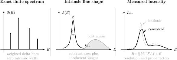
Three different objects. A finite closed system has exact weighted delta lines. A limiting procedure can produce an intrinsic quasiparticle peak of coherent area $Z$ plus continuum weight. A detector records a matrix-element- and occupation-weighted convolution with resolution $R$, often with background $B$.

Spectral Weight Is Area

For the normalized Lorentzian,

$$\int_{-\infty}^{\infty} dE\, L_\gamma(E-E_\star) = 1.$$

Therefore the coherent contribution

$$ZL_\gamma(E-E_\star)$$

has integrated area $Z$ for every $\gamma\gt0$. Its height,

$$\frac{Z}{\pi\gamma},$$

changes when the width changes. Comparing peak heights without comparing widths can therefore reverse the conclusion about spectral weight.

Coherent and incoherent decomposition

A useful local decomposition is

$$A(\mathbf k,E) = A_{\mathrm{coh}}(\mathbf k,E) + A_{\mathrm{inc}}(\mathbf k,E).$$

For one canonical orbital,

$$\int dE\, A(\mathbf k,E) = 1.$$

If one coherent pole has weight $Z_{\mathbf k}$, then

$$\int dE\, A_{\mathrm{inc}}(\mathbf k,E) = 1-Z_{\mathbf k}$$

only when all other coherent poles have been excluded from the definition of $A_{\mathrm{inc}}$. In multiband or symmetry-broken problems, several coherent branches may share the total weight.

Partial windows

Experiments and computations integrate over finite windows:

$$W(E_1,E_2) = \int_{E_1}^{E_2} dE\, A(E).$$

A change in $W$ can mean:

• true transfer of weight across the window boundary;
• a shifting peak;
• temperature-dependent occupation;
• a matrix-element change;
• resolution leakage;
• background subtraction;
• unmeasured tails.

It is not automatically a violation of a sum rule.

Moment constraints

Zeroth moments test normalization. Higher moments test commutators, kinetic energy, interactions, and asymptotic expansions. Sum Rules develops those exact constraints. Here the practical rule is:

Every reported loss of spectral weight must name the integration measure, window, operator channel, normalization, and missing destination.

Worked Benchmark: Free Fermion

For

$$\mathcal K = \sum_{\mathbf k} \xi_{\mathbf k} c_{\mathbf k}^\dagger c_{\mathbf k},$$

the retarded Green function is

$$G_0^{\mathrm R}(\mathbf k,E) = \frac1{ E-\xi_{\mathbf k}+i0^+ }.$$

Therefore

$$A_0(\mathbf k,E) = \delta \left( E-\xi_{\mathbf k} \right).$$

The excitation is perfectly sharp, has residue one, and follows the bare dispersion. Its occupied removal intensity at equilibrium is nevertheless weighted by

$$f(E) = \frac1{ e^{\beta E}+1 }.$$

A state above the chemical potential can be present in $A$ but absent from an ideal removal spectrum at zero temperature. Spectrum and occupation are different data.

Worked Benchmark: BCS Coherence Peaks

For a translationally invariant BCS saddle, the electron spectral function is

$$\begin{aligned} A(\mathbf k,E) ={}& u_{\mathbf k}^2 \delta(E-E_{\mathbf k}) \\ &+ v_{\mathbf k}^2 \delta(E+E_{\mathbf k}), \end{aligned}$$

where

$$E_{\mathbf k} = \sqrt{ \xi_{\mathbf k}^2 + |\Delta_{\mathbf k}|^2 }.$$

The coherence factors satisfy

$$u_{\mathbf k}^2 + v_{\mathbf k}^2 = 1.$$

The two branches therefore split one unit of canonical electron weight. At zero temperature,

$$n_{\mathbf k} = \int_{-\infty}^{0} dE\, A(\mathbf k,E) = v_{\mathbf k}^2.$$

The negative-energy peak is not a negative-norm state. It is particle-removal weight created by particle–hole mixing. BCS Mean-Field Theory owns the Bogoliubov transformation and coherence-factor derivation.

Bogoliubov Quasiparticles explains why these pole weights are canonical coherence factors, how they differ from an interaction-renormalized residue, and why bosonic commutator spectra instead carry signed negative-frequency weight.

Interactions beyond the saddle can broaden the peaks, shift their energies, create satellites, and transfer weight into continua. A broadened two-peak fit alone does not establish weak-coupling BCS physics.

Energy and Momentum Cuts

A two-dimensional spectral map

$$A(\mathbf k,E)$$

is commonly analyzed through two kinds of cuts.

Energy-distribution curve

An energy-distribution curve holds momentum fixed and scans $E$. Its line shape directly samples the energy dependence of the self-energy, matrix element, occupation factor, and background at that momentum.

Momentum-distribution curve

A momentum-distribution curve holds $E$ fixed and scans momentum. If the dispersion is locally linear,

$$E-E_{\mathbf k}^\star \simeq - \mathbf v^\star \cdot (\mathbf k-\mathbf k_\star),$$

and if the self-energy and matrix element vary weakly with momentum, the momentum HWHM is approximately

$$\Delta k_{\mathrm{HWHM}} \simeq \frac{\gamma}{ |\mathbf v^\star| }.$$

This conversion fails near a band extremum, flat band, strong momentum-dependent self-energy, overlapping band, or matrix-element zero. An energy width and momentum width are not interchangeable without a local dispersion model.

From Intrinsic Spectrum to Measured Intensity

A useful schematic forward model is

$$\begin{aligned} I_{\mathrm{obs}}(x,E) ={}& \int dx'\,dE'\, R_x(x-x') R_E(E-E') \\ &\times |M(x',E')|^2 \mathcal F(E') \mathcal S(x',E') \\ &+ B(x,E). \end{aligned}$$

Here:

• $x$ denotes momentum, position, angle, polarization, or another resolved variable;
• $\mathcal S$ is the intrinsic operator spectrum;
• $M$ is a probe matrix element;
• $\mathcal F$ is an occupation or detailed-balance factor;
• $R_x$ and $R_E$ are normalized resolution kernels;
• $B$ is background.

The appropriate $\mathcal S$ and $\mathcal F$ depend on the experiment.

Removal spectroscopy

Photoemission, radio-frequency ejection, and related removal probes can approach

$$I_{\mathrm{rem}}(\mathbf k,E) \propto |M(\mathbf k,E)|^2 f(E) A(\mathbf k,E),$$

before final-state effects, escape depth, kinematic factors, and resolution are included.

At zero temperature, $f(E)$ suppresses positive-energy addition weight. Dividing noisy data by a small Fermi factor is not a model-independent reconstruction of the unoccupied spectrum.

Addition spectroscopy

Inverse photoemission or injection probes can emphasize

$$I_{\mathrm{add}}(\mathbf k,E) \propto |M(\mathbf k,E)|^2 \left[ 1-f(E) \right] A(\mathbf k,E).$$

Addition and removal experiments need not have the same matrix elements, backgrounds, or final-state broadening.

Tunneling spectroscopy

In a weak-tunneling limit, current involves a convolution of tip and sample spectral densities:

$$\begin{aligned} I(V) \propto \int dE\, &\nu_{\mathrm{tip}}(E-eV) \nu_{\mathrm{sample}}(E) \\ &\times \left[ f(E-eV)-f(E) \right] |T(E,V)|^2. \end{aligned}$$

The often-used approximation

$$\frac{dI}{dV} \propto \nu_{\mathrm{sample}}(eV)$$

requires a sufficiently featureless tip, weak tunneling, controlled voltage drop, low enough temperature, and slowly varying matrix element. It is not a universal identity.

Scanning Tunneling Microscopy and Spectroscopy owns the operating junction, feedback and setpoint effects, conductance mapping, quasiparticle interference, and experimental calibration.

Scattering spectroscopy

Neutron, X-ray, electron, and cold-atom Bragg probes transfer momentum and energy without adding the same constituent whose single-particle propagator defines $A$. Their intrinsic target object is commonly a dynamic structure factor or susceptibility:

$$S_O(\mathbf q,E)$$

or

$$\chi_{OO}^{\mathrm R}(\mathbf q,E).$$

Polarization factors, form factors, kinematics, and detailed balance multiply the target spectrum. A mode seen in scattering and a peak seen in photoemission may arise from related physics while remaining different operator channels.

Matrix-element zeros

If

$$M(x,E) = 0,$$

the measured intensity vanishes even when the intrinsic spectrum is nonzero. Changing photon energy, polarization, probe geometry, tip orbital, or transferred momentum can therefore make a feature appear or disappear without changing the target Hamiltonian.

Resolution convolution

Even normalized resolution kernels preserve total weight only when the full domain is integrated:

$$\int dE\, R_E(E-E') = 1.$$

Finite detector windows, nonlinear calibration, clipping, and background subtraction can spoil apparent conservation. Deconvolution amplifies noise and is not unique without regularization or prior information.

Numerical Spectra

This section records the interpretation of common numerical outputs. Dynamical Correlation Functions Numerically gives the full comparative workflow, common benchmark, resolution ledger, and reporting standard.

Exact diagonalization

Finite exact diagonalization produces weighted delta functions. A common display replaces

$$\delta(E-E_j)$$

by

$$L_\eta(E-E_j) = \frac1\pi \frac{\eta}{ (E-E_j)^2+\eta^2 }.$$

The integrated weight is preserved, but peak height, apparent overlap, and gap visibility depend on $\eta$. A convergence study should vary:

• system size;
• boundary conditions;
• symmetry sector;
• broadening kernel;
• broadening width;
• frequency window.

For a sparse Hamiltonian, Lanczos Method Preview shows how the operator-generated seed $A|0\rangle$ yields a tridiagonal continued fraction, why the response run can occupy a different symmetry sector, and which residual and moment checks belong in the numerical record.

Real-time calculation

A record of duration $T$ has characteristic energy resolution

$$\Delta E \sim \frac{2\pi\hbar}{T}.$$

A rectangular time window produces sinc-like ringing. Smooth windows reduce sidelobes but broaden the main lobe and convolve the true spectrum with the window transform. Zero padding interpolates the plotted frequency grid; it does not increase physical resolution.

Imaginary-time continuation

Imaginary-time or Matsubara data constrain a smoothed integral transform of the real-frequency spectrum. Recovering narrow lines, nearby peaks, or sharp thresholds from finite noisy data is ill conditioned.

A continuation result should report:

1. the data covariance and fitted residuals;
2. the positivity assumption and whether it is valid for the channel;
3. exact normalization and known moments;
4. prior or regularizer dependence;
5. synthetic-data resolution tests;
6. stability under removing imaginary-time or Matsubara points;
7. uncertainty on integrated features, not only a smooth central curve.

Two reconstructions that fit the imaginary-axis data equally well can disagree on linewidths smaller than the continuation resolution.

Analytic Continuation is the canonical home for covariance whitening, singular-value resolution, method families, synthetic tests, and ambiguity-aware reporting. This page retains the physical interpretation of whatever spectral structure survives those tests.

Correction-vector and resolvent methods

After shifting by a declared reference energy $E_{\mathrm{ref}}$, methods that evaluate

$$\langle\psi| O \frac1{ E+i\eta-(H-E_{\mathrm{ref}}) } O^\dagger |\psi\rangle$$

compute an $\eta$-broadened object directly. The linear-solver tolerance, variational truncation, finite size, and $\eta$ all contribute errors. Extrapolating $\eta\to0^+$ is a separate limiting problem.

Comparing Theory and Experiment

A useful comparison matches more than peak position.

When the baseline is a crystal band calculation, Band Structure Workflows owns the converged Kohn–Sham or model-band object and its provenance. This page owns the distinct many-body spectral object, coherent and incoherent weight, line shapes, and the forward comparison with measured intensity.

DMFT for Quantum Materials owns the material calculation that produces validated interacting Green functions and continuation-bounded spectral estimates within its declared local-self-energy model. This page retains the interpretation of those spectral features and their experimental forward model.

Forward comparison

Prefer applying the experimental forward model to the theoretical spectrum:

$$\mathcal S_{\mathrm{theory}} \longrightarrow I_{\mathrm{predicted}},$$

then compare $I_{\mathrm{predicted}}$ with raw or minimally processed data. This keeps resolution, occupation, matrix elements, and background assumptions explicit.

Quantities to compare

At minimum compare:

• peak or threshold energy;
• integrated weight over declared windows;
• intrinsic and observed widths separately;
• momentum dispersion;
• temperature and control-parameter dependence;
• polarization or channel dependence;
• asymmetry and continuum shape;
• exact moments available to both sides.

Agreement in one peak position does not establish agreement in spectral function.

Uncertainty propagation

Fit uncertainties should include correlations among:

• energy calibration;
• resolution width;
• background parameters;
• matrix-element model;
• occupation temperature;
• overlapping peaks;
• finite-window tails.

Subtracting a flexible background can trade continuum weight for peak area. That covariance should be reported rather than hidden by a single best-fit curve.

Validation Checklist

Before interpreting a spectral feature, verify:

1. Object: Is the plotted quantity $A$, $S$, $\rho$, $\nu$, $J$, or measured intensity?
2. Operators: Which insertion creates and which detects the excitation?
3. State: Ground state, thermal equilibrium, driven state, or ensemble average?
4. Energy zero: Absolute energy, chemical potential, elastic line, or another reference?
5. Transform: Energy or angular frequency, with which $2\pi$ and $\hbar$ factors?
6. Normalization: What exact zeroth moment should be recovered?
7. Positivity: Is positivity valid for this ordered channel or only for a matrix quadratic form?
8. Limits: Finite size, thermodynamic limit, isolated system, open system, or disorder average?
9. Width: Intrinsic self-energy, plotting $\eta$, finite-time window, resolution, or inhomogeneity?
10. Forward model: Which matrix elements, occupations, form factors, and backgrounds intervene?
11. Moments: Does the spectrum satisfy known equal-time and high-frequency constraints?
12. Robustness: Are positions, areas, and widths stable under fit-window and resolution changes?

Common Mistakes

Calling every maximum a quasiparticle

A maximum can arise from a threshold, overlapping continuum, matrix-element variation, or resolution convolution. A quasiparticle claim requires a controlled pole region and consistent dispersion.

Reading peak height as residue

Residue is coherent integrated weight. Height depends inversely on width for a Lorentzian and also depends on resolution.

Treating finite broadening as a lifetime

The numerical parameter $\eta$ and the retarded $i0^+$ prescription do not establish physical decay.

Ignoring the operator

Different operators see different subsets of the exact spectrum. A dark state in one channel can be bright in another.

Calling the density of states the spectral function

The density of states is a trace or momentum integral of a spectral function under specified conventions. It has discarded momentum and often orbital information.

Equating intensity with intrinsic spectrum

Measured counts include matrix elements, occupations, resolution, background, and sometimes substantial final-state effects.

Assuming all spectral densities are positive

Ordered conjugate spectra and fermionic $A$ are positive in the appropriate sense. Commutator response densities and off-diagonal components can be signed or complex.

Ignoring negative-energy conventions

Negative energy can mean removal relative to $\mu$, target de-excitation, or a reversed Fourier convention. The axis label must identify which.

Fitting a Lorentzian across a threshold

Energy-dependent self-energy and phase-space edges generate non-Lorentzian shapes. A narrow fit uncertainty does not repair a wrong model.

Declaring missing weight without a destination

Weight can move outside the measured window, into another branch, into a continuum, or behind a matrix-element zero. A sum-rule claim requires full normalization bookkeeping.

Confusing one-particle and collective momentum

$A(\mathbf k,E)$ resolves the momentum of an added or removed particle. $S(\mathbf q,E)$ resolves momentum transferred by a number-preserving probe.

Overinterpreting analytic continuation

A smooth reconstructed curve can conceal nonuniqueness. Features narrower than the demonstrated continuation resolution should not be quoted as resolved.

Reliable Workflow

1. Write the operator correlation or Green function before naming its spectrum.
2. State the state, generator, energy zero, transform, and normalization.
3. Derive or quote the Lehmann weights and identify their positivity properties.
4. Separate pure-point lines from continuous support before applying broadening.
5. Test exact zeroth and known higher moments.
6. Identify candidate poles, thresholds, and symmetry-forced zeros.
7. Fit a quasiparticle only where the self-energy and background are locally smooth.
8. Report HWHM or FWHM explicitly and separate every broadening source.
9. Apply occupation, matrix-element, form-factor, resolution, and background models to compare with experiment.
10. Vary size, window, kernel, fit range, and regularization to expose systematic uncertainty.

Exercises

Exercise 1: Lorentzian weight and delta limit

For

$$L_\gamma(E-E_0) = \frac1\pi \frac{\gamma}{ (E-E_0)^2+\gamma^2 }, \qquad \gamma\gt0,$$

show that its integral is one, identify its HWHM and FWHM, and explain the sense in which it approaches $\delta(E-E_0)$ as $\gamma\to0^+$.

Solution

Set

$$x = \frac{E-E_0}{\gamma}.$$

Then

$$\begin{aligned} \int_{-\infty}^{\infty} dE\, L_\gamma(E-E_0) &= \frac1\pi \int_{-\infty}^{\infty} \frac{dx}{1+x^2} \\ &= 1. \end{aligned}$$

The maximum is

$$L_\gamma(0) = \frac1{\pi\gamma}.$$

Half the maximum occurs at

$$|E-E_0| = \gamma.$$

Thus

$$\operatorname{HWHM} = \gamma, \qquad \operatorname{FWHM} = 2\gamma.$$

For every smooth test function $f$ that varies slowly enough near $E_0$,

$$\lim_{\gamma\to0^+} \int dE\, L_\gamma(E-E_0)f(E) = f(E_0).$$

That distributional statement, rather than pointwise convergence at $E_0$, defines the delta limit.

Exercise 2: Bright and dark exact states

A ground state $|0\rangle$ and two excited states $|1\rangle$, $|2\rangle$ have excitation energies $\Delta_1$ and $\Delta_2$. Suppose

$$O^\dagger|0\rangle = \sqrt w\,|1\rangle, \qquad 0\leq w\leq1,$$

and $\langle2|O^\dagger|0\rangle=0$. Find the zero-temperature transition spectrum and explain what can and cannot be inferred from the missing line at $\Delta_2$.

Solution

The Lehmann representation gives

$$\mathcal S_{O O^\dagger}(E) = w\, \delta(E-\Delta_1).$$

There is no line at $\Delta_2$ because the matrix element vanishes. One may infer that state $|2\rangle$ is dark to this operator in this reference state. One may not infer that $|2\rangle$ is absent from the Hamiltonian spectrum. A different operator, momentum, or polarization may couple to it.

The total weight is

$$\int dE\, \mathcal S_{O O^\dagger}(E) = w = \langle0|OO^\dagger|0\rangle.$$

It need not be one because $O$ was not assumed to be a canonical fermion operator.

Exercise 3: BCS weight and occupation

Given

$$A(\mathbf k,E) = u_{\mathbf k}^2\delta(E-E_{\mathbf k}) + v_{\mathbf k}^2\delta(E+E_{\mathbf k}),$$

with $E_{\mathbf k}\gt0$ and $u_{\mathbf k}^2+v_{\mathbf k}^2=1$, verify the fermionic zeroth moment and compute $n_{\mathbf k}$ at zero temperature.

Solution

Integration over all energies gives

$$\begin{aligned} \int_{-\infty}^{\infty} dE\, A(\mathbf k,E) &= u_{\mathbf k}^2 + v_{\mathbf k}^2 \\ &= 1. \end{aligned}$$

At zero temperature the occupied side is $E\lt0$, so

$$\begin{aligned} n_{\mathbf k} &= \int_{-\infty}^{0} dE\, A(\mathbf k,E) \\ &= v_{\mathbf k}^2. \end{aligned}$$

The positive-energy peak carries addition weight $u_{\mathbf k}^2$; the negative-energy peak carries removal weight $v_{\mathbf k}^2$.

Exercise 4: Linearized self-energy

Consider

$$\Sigma^{\mathrm R}(E) = \Sigma_0 + \left( 1-Z_0^{-1} \right)E - i\frac{\gamma_0}{Z_0},$$

with real $\Sigma_0$, $0\lt Z_0\leq1$, and $\gamma_0\gt0$. For a bare level $\xi$, find the renormalized energy, residue, and Lorentzian HWHM.

Solution

The pole equation is

$$E^\star - \xi - \Sigma_0 - \left( 1-Z_0^{-1} \right)E^\star = 0.$$

Therefore

$$E^\star = Z_0 \left( \xi+\Sigma_0 \right).$$

The derivative formula gives

$$\begin{aligned} Z &= \left[ 1- \left( 1-Z_0^{-1} \right) \right]^{-1} \\ &= Z_0. \end{aligned}$$

Finally,

$$\gamma = - Z\operatorname{Im}\Sigma^{\mathrm R} = - Z_0 \left( -\frac{\gamma_0}{Z_0} \right) = \gamma_0.$$

The spectral FWHM is $2\gamma_0$, provided the linearized form remains valid across that width.

Exercise 5: Two-particle threshold exponent

For two particles in $d$ dimensions with

$$\epsilon(\mathbf p) = \Delta + \frac{\mathbf p^2}{2m},$$

derive the threshold at fixed total momentum $\mathbf q$ and show that a constant matrix element gives near-threshold weight proportional to $(E-E_{\mathrm{th}})^{d/2-1}$.

Solution

Use relative momentum $\mathbf p$:

$$\mathbf p_{1,2} = \frac{\mathbf q}{2} \pm \mathbf p.$$

Then

$$\epsilon(\mathbf p_1) + \epsilon(\mathbf p_2) = 2\Delta + \frac{\mathbf q^2}{4m} + \frac{\mathbf p^2}{m}.$$

The minimum occurs at $\mathbf p=\mathbf0$, so

$$E_{\mathrm{th}}(\mathbf q) = 2\Delta + \frac{\mathbf q^2}{4m}.$$

Let

$$\varepsilon = E-E_{\mathrm{th}}.$$

The phase-space integral is

$$\int d^dp\, \delta \left( \varepsilon-\frac{\mathbf p^2}{m} \right).$$

In spherical coordinates it scales as

$$p^{d-1} \left| \frac{d(p^2/m)}{dp} \right|^{-1} \propto p^{d-2}.$$

Since $p\propto\sqrt\varepsilon$,

$$\mathcal S(E) \propto \varepsilon^{d/2-1} \Theta(\varepsilon).$$

A matrix element that vanishes as $p^\ell$ contributes an additional power $\varepsilon^\ell$ after squaring the amplitude.

Exercise 6: Resolution broadening

An intrinsic Lorentzian has HWHM $\gamma_{\mathrm{int}}$. The detector response is another normalized Lorentzian with HWHM $\gamma_{\mathrm{res}}$. What observed width results? How would the rule change for two Gaussian profiles?

Solution

The convolution of two Lorentzians is Lorentzian, with HWHM values adding:

$$\gamma_{\mathrm{obs}} = \gamma_{\mathrm{int}} + \gamma_{\mathrm{res}}.$$

Equivalently, their FWHM values add.

For Gaussian profiles, variances add:

$$\sigma_{\mathrm{obs}}^2 = \sigma_{\mathrm{int}}^2 + \sigma_{\mathrm{res}}^2.$$

Because Gaussian FWHM is proportional to $\sigma$, Gaussian FWHM values add in quadrature, not linearly. A Lorentzian convolved with a Gaussian gives a Voigt profile, so neither simple rule is exact for the resulting FWHM.

Exercise 7: Finite time and artificial linewidth

A real-time calculation reaches $T=200\,\hbar/J$, where $J$ is an energy scale. Estimate the characteristic energy resolution. Explain why zero padding cannot resolve two lines separated by $0.01J$.

Solution

The characteristic resolution is

$$\Delta E \sim \frac{2\pi\hbar}{T} = \frac{2\pi}{200}J \approx 0.031J.$$

Two lines separated by $0.01J$ lie within this main resolution scale. Zero padding inserts additional frequency-grid points between the original discrete transform samples, making the curve look smoother. It does not add late-time information and therefore cannot create the missing resolving power.

A different window can alter ringing and numerical peak width, but resolving the pair requires a longer reliable time record or independent prior information.

Exercise 8: Choose the spectral object

For each task, identify the most direct intrinsic object and one forward-model factor that must still be considered:

1. remove an electron with angle-resolved photoemission;
2. scatter neutrons from spin fluctuations;
3. infer local electronic states with a tunneling tip;
4. model a qubit coupled to oscillator bath modes.

Solution

1. Use the fermionic removal part of $A(\mathbf k,E)$. The Fermi factor, photoemission matrix element, final state, and instrumental resolution intervene.
2. Use the spin dynamic structure factor $S^{\alpha\beta}(\mathbf q,E)$ or the related susceptibility. Magnetic form factors and polarization projectors intervene.
3. Use local sample and tip spectral densities in the tunneling-current convolution. The tunneling matrix element, tip density of states, temperature, and voltage drop intervene.
4. Use the bath coupling spectral density $J(\omega)$. The system coupling operator and thermal occupation factors intervene.

The objects can share similar line shapes, but their operators and normalizations are different.

Cross-Links

• Unconventional Superconductivity places momentum-resolved gap and coherence information into a crystal-symmetry and multi-probe evidence audit; this page retains the generic spectral object, sum rules, linewidths, and measured-intensity firewall.
• How Quantum Matter Is Measured distinguishes an intrinsic spectral object from the matrix elements, acceptance, resolution, and reduction steps that produce measured intensity.
• Angle-Resolved Photoemission Spectroscopy turns occupied removal weight into a solid-state momentum-mapping experiment with explicit kinematics, surface, matrix-element, resolution, and calibration controls.
• Photoelectron Spectroscopy — experimental energy references, matrix elements, escape-depth effects, and the limits of identifying photoemission intensity directly with removal spectral weight.
• Edge and Surface States — projected bulk gaps, boundary spectral functions, surface-sensitive probes, and the distinction between a visible boundary band and topological protection.
• Green Functions in Many-Body QM — full single-particle Lehmann, positivity, normalization, and Dyson derivations.
• Retarded and Advanced Response — commutator spectral density, analyticity, and dispersion relations.
• Spectral Representation — exact thermal kernels connecting Euclidean, Matsubara, and retarded functions.
• Structure Factors — momentum-transfer spectra and scattering forward models.
• Time-Dependent Correlations — finite-time records, recurrence, dephasing, and Fourier windows.
• Susceptibilities — named response channels, units, and measurement protocols.
• Kubo Formula — source-to-response derivation.
• Fluctuation–Dissipation Theorem — equilibrium detailed balance, quantum factors, and classical limits.
• Sum Rules — exact integrated constraints and numerical saturation tests.
• Lanczos Method Preview — Krylov ground states, continued-fraction spectra, and finite-precision checks.
• Dynamical Correlation Functions Numerically — matched Lehmann, resolvent, and real-time estimators with explicit resolution control.
• Spectral Representation of Green Functions — resolvent and spectral-theorem foundations.
• Green Functions and Density of States — local and total state-counting formulas.
• Anderson Insulators — why finite single-particle density of states can coexist with zero diffusion, and how a soft Coulomb gap modifies hopping transport.
• Mobility Edges — why an energy-resolved localization transition need not create a spectral gap or singular average density of states.
• Diagrammatic Methods Preview — proper self-energy insertions and Dyson resummation.
• Fermi Liquid Theory Preview — finite residue, quadratic low-energy width, Landau parameters, and quasiparticle response.
• BCS Mean-Field Theory — Bogoliubov branches and coherence factors.
• Anderson Impurity Model Preview — resonant-level, hybridization, and correlated atomic spectra.
• Energy-Time Uncertainty — bounded lifetime–linewidth statements.
• Spectral Densities — coupling-weighted reservoir spectra.
• Correlation Functions Formula Card — compact ordering and normalization lookup.
• Fourier-Transform Conventions — energy and angular-frequency transforms.

References

1. H. Lehmann, “Über Eigenschaften von Ausbreitungsfunktionen und Renormierungskonstanten quantisierter Felder”, Il Nuovo Cimento 11, 342–357 (1954).
2. F. J. Dyson, “The Radiation Theories of Tomonaga, Schwinger, and Feynman”, Physical Review 75, 486–502 (1949).
3. J. M. Luttinger, “Analytic Properties of Single-Particle Propagators for Many-Fermion Systems”, Physical Review 121, 942–949 (1961).
4. J. J. Quinn and R. A. Ferrell, “Electron Self-Energy Approach to Correlation in a Degenerate Electron Gas”, Physical Review 112, 812–827 (1958).
5. U. Fano, “Effects of Configuration Interaction on Intensities and Phase Shifts”, Physical Review 124, 1866–1878 (1961).
6. J. Bardeen, “Tunnelling from a Many-Particle Point of View”, Physical Review Letters 6, 57–59 (1961).
7. J. Tersoff and D. R. Hamann, “Theory and Application for the Scanning Tunneling Microscope”, Physical Review Letters 50, 1998–2001 (1983).
8. J. Bardeen, L. N. Cooper, and J. R. Schrieffer, “Theory of Superconductivity”, Physical Review 108, 1175–1204 (1957).
9. A. W. Sandvik, “Stochastic Method for Analytic Continuation of Quantum Monte Carlo Data”, Physical Review B 57, 10287–10290 (1998).
10. A. L. Fetter and J. D. Walecka, Quantum Theory of Many-Particle Systems, Dover (2003).
11. G. D. Mahan, Many-Particle Physics, 3rd ed., Springer (2000).
12. P. Coleman, Introduction to Many-Body Physics, Cambridge University Press (2015).
13. E. N. Economou, Green’s Functions in Quantum Physics, 3rd ed., Springer (2006).
14. S. Hüfner, Photoelectron Spectroscopy: Principles and Applications, 3rd ed., Springer (2003).