Transport Coefficients Preview

A transport coefficient quantifies the response of a flux to a weak, slowly varying drive near equilibrium. Electrical conductivity relates charge current to electric field, a diffusion constant relates conserved-density gradients to particle flow, and viscosity relates momentum flux to velocity gradients. These coefficients are macroscopic, but equilibrium correlation functions provide microscopic formulas for them.

The central chain of reasoning is

$$\begin{gathered} \text{conservation law} \\ \quad+\quad \text{constitutive relation} \\ \Longrightarrow \text{hydrodynamic pole}, \\ \text{linear response} \\ \quad+\quad \text{equilibrium correlations} \\ \Longrightarrow \text{Kubo or Green–Kubo relation}. \end{gathered}$$

The two routes must agree when the same variables, sources, limits, and normalizations are used. Their agreement is a stringent check; it is not automatic in a finite isolated system or in a model whose relevant current cannot relax.

This page is a bridge. It organizes the generic coefficients, their physical meanings, and the limits needed to extract them. It does not repeat the source derivation and electromagnetic contact terms developed on Kubo Formula, the density and current construction on Density Operators and Current Operators, or the exact integrated constraints on Sum Rules.

For material-specific model selection and probe-facing response, continue through Transport, Response, and Optics.

Canonical Scope

This page owns:

• the generic dictionary among currents, thermodynamic forces, and transport coefficients;
• diffusion from a conservation law and a constitutive relation;
• the diffusion pole and its noncommuting static and uniform limits;
• the Einstein relation among conductivity, compressibility, and diffusion;
• Green–Kubo formulas and their convergence conditions;
• a preview of thermoelectric response, shear viscosity, bulk viscosity, and sound attenuation;
• ballistic, diffusive, anomalous, and localized transport regimes;
• the order-of-limits and finite-size logic needed to interpret dc response;
• the bridge from microscopic correlation functions to hydrodynamic modes.

Neighboring canonical homes retain narrower subjects:

• Kubo Formula owns the source-response derivation, Lehmann representation, electromagnetic contact term, and full optical-conductivity formula.
• Fluctuation–Dissipation Theorem owns the KMS conversion between noise and absorption.
• Density Operators and Current Operators owns local densities, continuum and lattice currents, and continuity equations.
• Collective Modes owns the broader classification of propagating, diffusive, underdamped, and overdamped collective poles; this page owns transport coefficients and their hydrodynamic extraction.
• Plasmons Preview owns how longitudinal conductivity and charge conservation enter dielectric zeros and plasma modes.
• Lifetime and Spectral Weight owns the distinction among single-particle, transport, coherence, energy-relaxation, and escape times.
• Mesoscopic Transport owns leads, reservoirs, tunneling rates, shot noise, and counting statistics in open devices.
• Material-specific resistivity, Hall response, thermopower, and phase phenomenology belong with the relevant Quantum Matter system.
• Hydrodynamics and Effective Theory Preview owns slow-variable selection, constitutive and fluctuation expansions, coupled conserved fields, nonlinear hydrodynamics, and the effective-field-theory handoff.

What a Coefficient Actually Specifies

A statement such as “the conductivity is finite” is incomplete. A transport coefficient is attached to a protocol:

Ingredient	Question that must be answered
transported quantity	number, charge, spin, energy, heat, or momentum?
flux	local current density, total current, or boundary current?
drive	electric field, chemical-potential gradient, temperature gradient, strain rate, or boundary bias?
state	equilibrium ensemble, temperature, chemical potential, and symmetry sector?
tensor channel	longitudinal, transverse, Hall, shear, or bulk?
geometry	infinite bulk, periodic cell, open sample, or lead-coupled device?
limit	which of volume, wave number, frequency, time, and regulator is taken first?
normalization	per volume, per area, per layer, or total conductance?

Conductivity and conductance are not interchangeable. In a homogeneous bulk sample,

$$j_\alpha = \sum_\beta \sigma_{\alpha\beta} E_\beta$$

defines a conductivity tensor. A two-terminal relation

$$I = G\,\Delta V$$

defines a conductance and includes geometry, contacts, and boundary conditions. The open-device problem belongs to mesoscopic transport even when a bulk conductivity helps interpret it.

Conventions Used Here

Let

$$\beta = \frac{1}{k_B T}.$$

The Fourier transform follows the response pages:

$$X(\mathbf q,\omega) = \int dt \int d^d r\, e^{i\omega t-i\mathbf q\cdot\mathbf r} X(\mathbf r,t).$$

Therefore

$$\partial_t \longrightarrow -i\omega, \qquad \nabla \longrightarrow i\mathbf q.$$

Retarded poles lie below the real axis. A diffusive mode consequently has

$$\omega_{\mathrm{diff}} = -iDq^2, \qquad D\gt0.$$

The retarded susceptibility convention is

$$\chi_{AB}^R(t) = \frac{i}{\hbar} \theta(t) \langle[A(t),B(0)]\rangle.$$

For a passive equilibrium state and a Hermitian diagonal channel,

$$\operatorname{Im} \chi_{AA}^R(\omega) \geq 0 \qquad (\omega\gt0).$$

This sign matters in the low-frequency formulas below. Literature using $-i\theta(t)$ for the retarded function carries the opposite sign in its imaginary part.

Conservation Laws and Constitutive Relations

Suppose a scalar density $n(\mathbf r,t)$ is locally conserved:

$$\partial_t n + \nabla\boldsymbol\cdot\mathbf j_N = 0.$$

This identity alone does not say how $\mathbf j_N$ depends on the state. Hydrodynamics adds a constitutive relation: an expansion of the current in slowly varying fields and their gradients. For an isotropic system with no background flow, the leading dissipative term is Fick’s law,

$$\mathbf j_N = -D\nabla n.$$

Combining the two equations gives

$$\partial_t n = D\nabla^2 n.$$

The separation is conceptually important:

• the continuity equation follows from a symmetry and is exact for the stated Hamiltonian;
• the constitutive relation is a long-wavelength, late-time approximation;
• the coefficient $D$ contains microscopic collision, scattering, or dephasing information;
• higher gradients and additional slow variables correct the leading diffusion equation.

If the density couples strongly to energy, momentum, an order parameter, or another conserved charge, a one-component Fick law is generally insufficient. The correct hydrodynamic variables must be retained before any mode is called diffusive.

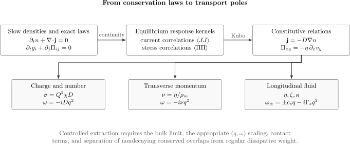
Transport connects three descriptions. Conservation laws identify slow densities and their fluxes. Equilibrium current or stress correlations determine kinetic coefficients. Constitutive relations then place those coefficients in diffusive, shear, and sound poles. Contact terms, conserved overlaps, and the order of $L$, $\mathbf q$, and $\omega$ limits belong to the map rather than being optional corrections.

Diffusion from a Density Source

Let an external chemical-potential source enter as

$$H_{\mathrm{pert}}(t) = -\int d^d r\, \delta\mu(\mathbf r,t) n(\mathbf r).$$

Write the equilibrium static susceptibility per volume as

$$\chi = \left( \frac{\partial n}{\partial\mu} \right)_T.$$

For small deviations, the intrinsic chemical-potential change is

$$\delta\mu_{\mathrm{int}} = \frac{\delta n}{\chi}.$$

A source $\delta\mu$ lowers the local free-energy cost of adding particles. The leading constitutive relation can therefore be written

$$\begin{aligned} \mathbf j_N &= -D\chi \nabla \left( \delta\mu_{\mathrm{int}} - \delta\mu \right) \\ &= -D\nabla\delta n + D\chi\nabla\delta\mu. \end{aligned}$$

Using continuity gives

$$\partial_t\delta n = D\nabla^2\delta n - D\chi\nabla^2\delta\mu.$$

Fourier transformation yields

$$\left( Dq^2-i\omega \right) \delta n(\mathbf q,\omega) = D\chi q^2 \delta\mu(\mathbf q,\omega).$$

Hence the hydrodynamic density response is

$$\chi_{nn}^R(\mathbf q,\omega) = \chi \frac{Dq^2} {Dq^2-i\omega}.$$

This compact expression encodes several distinct facts.

Pole and relaxation time

The pole occurs at

$$\omega = -iDq^2.$$

A modulation with wavelength of order $q^{-1}$ relaxes on the time scale

$$\tau_q = \frac{1}{Dq^2}.$$

Long-wavelength density variations relax slowly because particles must travel farther while total number remains conserved.

Absorptive density response

For real positive frequency,

$$\operatorname{Im} \chi_{nn}^R(\mathbf q,\omega) = \chi \frac{ Dq^2\omega }{ \left(Dq^2\right)^2+\omega^2 }.$$

It is nonnegative under the present retarded convention. Fluctuation–Dissipation Theorem converts this absorptive line shape into the corresponding equilibrium density-fluctuation spectrum.

Noncommuting limits

Taking the static limit first gives

$$\lim_{\mathbf q\to0} \lim_{\omega\to0} \chi_{nn}^R(\mathbf q,\omega) = \chi.$$

At exactly zero wave number, the perturbation couples to total particle number. Isolated finite-frequency dynamics cannot redistribute that conserved quantity:

$$\lim_{\omega\to0} \lim_{\mathbf q\to0} \chi_{nn}^R(\mathbf q,\omega) = 0.$$

The apparent contradiction is the signature of a hydrodynamic pole. The equilibrium compressibility and the uniform isolated response are different protocols.

Joint hydrodynamic scaling

Diffusion is not obtained by setting $\mathbf q=0$ at the start. Its scaling limit keeps

$$\frac{\omega}{Dq^2}$$

fixed while

$$q\longrightarrow0, \qquad \omega\longrightarrow0,$$

after a bulk limit has produced a sufficiently dense spectrum. This joint limit resolves the pole shape rather than collapsing it to either of the two static values.

Real-Space Spreading

For an initially localized conserved packet in an infinite isotropic medium, define

$$\mathcal N_D(t) = \frac{1} {\left(4\pi Dt\right)^{d/2}}.$$

The diffusion equation then has Green function

$$\begin{aligned} G(\mathbf r,t) &= \mathcal N_D(t) \exp \left( -\frac{r^2}{4Dt} \right), \\ &\hspace{2em} t\gt0. \end{aligned}$$

It is normalized:

$$\int d^d r\, G(\mathbf r,t) = 1.$$

Its mean-square displacement is

$$\langle r^2(t)\rangle = 2dDt.$$

This gives an independent operational definition of $D$. Agreement between packet spreading, the density-response pole, and a current-correlation formula is strong evidence that a genuine diffusive regime has been reached.

Boundary conditions modify the late-time profile. In a finite closed region, the density eventually approaches its conserved uniform mode rather than spreading forever.

Einstein Relation

The Einstein relation connects diffusion to response under a force. It is most transparent when chemical and electrical conventions are separated.

Let particles carry signed charge $Q$, and let

$$\widetilde\mu = \mu+Q\phi$$

be an electrochemical potential, with

$$\mathbf E = -\nabla\phi.$$

At fixed temperature, write the particle current as

$$\mathbf j_N = -\mathcal M \nabla\widetilde\mu,$$

where $\mathcal M$ is a number-transport coefficient. With no electric field,

$$\nabla\mu = \frac{1}{\chi} \nabla n,$$

so comparison with Fick’s law gives

$$D = \frac{\mathcal M}{\chi}.$$

With uniform chemical potential but nonzero electric field,

$$\mathbf j_N = \mathcal M Q\mathbf E.$$

The charge current is

$$\mathbf j_Q = Q\mathbf j_N = \sigma\mathbf E.$$

Therefore

$$\sigma = Q^2\chi D.$$

This relation uses:

• the susceptibility $\chi=(\partial n/\partial\mu)_T$ for the same conserved density;
• a common long-wavelength, low-frequency diffusive regime;
• local equilibrium and linear response;
• consistent number-current and charge-current normalizations.

For a dilute classical gas,

$$\chi = \frac{n}{k_BT},$$

so

$$\sigma = \frac{nQ^2D}{k_BT}.$$

If mechanical mobility $b$ is defined by drift velocity $\mathbf v_{\mathrm{drift}}=b\mathbf F$, then

$$D = b\,k_BT.$$

The symbols “mobility” and “compressibility” have several conventions. Stating their defining equations is safer than importing an Einstein relation by name.

Conductivity Dictionary

Electrical conductivity is a tensor:

$$j_\alpha(\mathbf q,\omega) = \sum_\beta \sigma_{\alpha\beta}(\mathbf q,\omega) E_\beta(\mathbf q,\omega).$$

Its symmetric longitudinal part dissipates energy. An antisymmetric Hall part can be nondissipative. In an isotropic system with no time-reversal-breaking field, the ordinary longitudinal response reduces to a scalar.

The full microscopic expression requires a current derived from the gauged Hamiltonian and, in general, a contact term. Under the conventions of Kubo Formula,

$$\sigma_{\alpha\beta}(\omega) = \frac{i}{\omega+i0} \left[ D_{\alpha\beta} - \Pi_{\alpha\beta}^R(\omega) \right].$$

Here $D_{\alpha\beta}$ is the diamagnetic or stress contribution and $\Pi^R$ is the paramagnetic current response per volume. This page uses that result but does not rederive it.

Reactive and dissipative parts

Write

$$\sigma(\omega) = \sigma'(\omega) + i\sigma''(\omega).$$

For a real monochromatic electric field, the cycle-averaged absorbed power density is proportional to

$$\sigma'(\omega) \lvert E(\omega)\rvert^2.$$

Passivity requires the dissipative quadratic form built from $\sigma'$ to be nonnegative. A Hall component does not contribute to

$$\mathbf E\boldsymbol\cdot\mathbf j$$

because its tensor is antisymmetric.

Drude and regular weight

A common bulk decomposition is

$$\operatorname{Re}\sigma(\omega) = \pi D_{\mathrm{Dr}} \delta(\omega) + \sigma_{\mathrm{reg}}(\omega).$$

A nonzero Drude weight represents a ballistic zero-frequency contribution under a stated order of limits. It is not a finite dc conductivity. In contrast, a regular diffusive conductor has

$$\sigma_{\mathrm{dc}} = \lim_{\omega\to0^+} \sigma_{\mathrm{reg}}(\omega)$$

finite after the bulk limit.

Interactions do not by themselves guarantee finite resistivity. If current overlaps a conserved momentum or another conserved quantity, part of the current can fail to decay. Disorder, umklapp, phonons, boundaries, or other relaxation channels may be required, depending on the model.

Relaxation-time benchmark

The Drude equation

$$\frac{d\mathbf j}{dt} + \frac{\mathbf j}{\tau} = \frac{nQ^2}{m} \mathbf E(t)$$

gives

$$\sigma(\omega) = \frac{nQ^2}{m} \frac{1} {\tau^{-1}-i\omega}.$$

Thus

$$\operatorname{Re}\sigma(\omega) = \frac{nQ^2\tau}{m} \frac{1} {1+\omega^2\tau^2},$$

and

$$\sigma_{\mathrm{dc}} = \frac{nQ^2\tau}{m}.$$

This is a benchmark, not an exact law for every interacting system. A single relaxation time can miss multiple slow modes, incoherent backgrounds, vertex corrections, localization, and frequency-dependent scattering.

Drude Theory is the canonical material-level treatment of this benchmark, including signed carriers, tensor masses, Hall response, optical spectral weight, transport versus quantum lifetimes, and fitting diagnostics.

Green–Kubo Relations

The retarded formula asks how a weak external source changes an observable. A Green–Kubo formula expresses a dc coefficient as an equilibrium time integral of spontaneous flux fluctuations.

For operators $A$ and $B$, define the Kubo-transformed canonical correlation

$$(A;B)_\beta = \frac{1}{\beta} \int_0^\beta d\lambda\, \left\langle \delta A(-i\hbar\lambda) \delta B \right\rangle,$$

where

$$\delta A = A-\langle A\rangle.$$

Let

$$\mathbf J_a = \int d^d r\, \mathbf j_a(\mathbf r)$$

be a total flux. For one Cartesian component in a homogeneous bulk system, a common Green–Kubo convention is

$$L_{ab} = \lim_{\mathrm{bulk}} \frac{1}{k_BV} \int_0^\infty dt\, \left( J_b; J_a(t) \right)_\beta.$$

The coefficient matrix $L$ relates fluxes to entropy-production forces defined below. In the classical limit, the Kubo transform reduces to the ordinary equilibrium correlation, giving

$$L_{ab}^{\mathrm{cl}} = \frac{1}{k_BV} \int_0^\infty dt\, \langle \delta J_b(0) \delta J_a(t) \rangle.$$

These compact formulas require qualifications:

• subtract equilibrium means and any nondecaying projected component;
• use the current associated with the same local conservation law and source;
• include contact or magnetization contributions when the physical response requires them;
• take the bulk limit before interpreting a continuous dc spectrum;
• verify convergence of the time integral;
• distinguish a true decay rate from numerical broadening;
• state whether the coefficient is longitudinal, transverse, open circuit, or constrained.

If the current correlation approaches a nonzero constant,

$$\lim_{t\to\infty} \frac{1}{V} \left( J;J(t) \right)_\beta \ne 0,$$

then the integral does not define an ordinary finite coefficient. The nondecaying part instead produces ballistic weight at zero frequency.

If the long-time tail behaves as

$$\frac{1}{V} \left( J;J(t) \right)_\beta \sim t^{-\alpha},$$

then the dc integral converges at its upper endpoint only for

$$\alpha\gt1.$$

At $\alpha=1$ it diverges logarithmically; for $\alpha\lt1$ it diverges as a power. Such tails can signal anomalous transport or the need to retain additional hydrodynamic modes.

Coupled Particle and Heat Transport

Transport channels can mix. For a one-component system, define the heat current by

$$\mathbf j_{\mathcal Q} = \mathbf j_E - \mu\mathbf j_N.$$

The precise definition can require additional magnetization or boundary subtractions in systems with magnetic fields, circulating currents, or nontrivial geometry.

The local entropy-production density contains

$$\begin{aligned} \dot s_{\mathrm{prod}} ={}& \mathbf j_N \boldsymbol\cdot \left[ -\nabla \left( \frac{\mu}{T} \right) \right] \\ &+ \mathbf j_{\mathcal Q} \boldsymbol\cdot \nabla \left( \frac{1}{T} \right) + \cdots. \end{aligned}$$

This motivates thermodynamic forces

$$\mathbf X_N = -\nabla \left( \frac{\mu}{T} \right), \qquad \mathbf X_{\mathcal Q} = \nabla \left( \frac{1}{T} \right).$$

Near equilibrium,

$$\begin{pmatrix} \mathbf j_N \\ \mathbf j_{\mathcal Q} \end{pmatrix} = \begin{pmatrix} L_{NN} & L_{N\mathcal Q} \\ L_{\mathcal QN} & L_{\mathcal Q\mathcal Q} \end{pmatrix} \begin{pmatrix} \mathbf X_N \\ \mathbf X_{\mathcal Q} \end{pmatrix}.$$

At uniform temperature, this convention gives

$$D = \frac{L_{NN}}{T\chi},$$

and, for particles of charge $Q$,

$$\sigma = \frac{Q^2L_{NN}}{T}.$$

Their ratio reproduces

$$\sigma = Q^2\chi D.$$

If the particle current is constrained to vanish, the scalar open-circuit thermal conductivity is

$$\kappa_{\mathbf j_N=0} = \frac{1}{T^2} \left( L_{\mathcal Q\mathcal Q} - \frac{ L_{\mathcal QN} L_{N\mathcal Q} }{ L_{NN} } \right).$$

The subtraction is physical: a temperature gradient can induce particle flow, and the compensating electrochemical field carries heat as well. Thermal conductivity measured at zero particle current therefore differs from the coefficient at zero electrochemical gradient.

Seebeck and Peltier coefficients are alternate parameterizations of the off-diagonal entries. Their signs and factors of $T$ depend on whether one uses particle, signed charge, energy, or heat current and on how the electrochemical potential is defined.

Onsager–Casimir Reciprocity and Positivity

Microscopic reversibility constrains coupled transport. Let $\varepsilon_a=\pm1$ denote the time-reversal parity associated with channel $a$. In a magnetic field or another time-reversal-odd background $\mathbf B$,

$$L_{ab}(\mathbf B) = \varepsilon_a\varepsilon_b L_{ba}(-\mathbf B).$$

At zero field, particle and energy transport in an ordinary time-reversal-invariant system give the familiar reciprocity

$$L_{N\mathcal Q} = L_{\mathcal QN}$$

under the force and flux conventions above.

Reciprocity is not the same as equality at fixed nonzero magnetic field. Hall and thermomagnetic coefficients are constrained by field reversal, not generally by a symmetric matrix at the same field.

The entropy-production rate requires the symmetric dissipative part of $L$ to be positive semidefinite:

$$\sum_{a,b} \mathbf X_a \boldsymbol\cdot L_{ab}^{(s)} \mathbf X_b \geq 0.$$

For the scalar two-channel matrix, this implies

$$L_{NN}\geq0, \qquad L_{\mathcal Q\mathcal Q}\geq0,$$

and

$$L_{NN} L_{\mathcal Q\mathcal Q} - L_{N\mathcal Q} L_{\mathcal QN} \geq 0$$

when the relevant symmetric matrix is used. The same determinant inequality ensures that the open-circuit thermal conductivity above is nonnegative.

Viscosity Preview

Viscosity is transport of momentum. Let $g_i$ be momentum density and $\Pi_{ij}$ the momentum-current or stress tensor. Local momentum conservation is

$$\partial_t g_i + \partial_j\Pi_{ij} = 0.$$

For an isotropic nonrelativistic fluid near rest, the leading constitutive relation is

$$\begin{aligned} \Pi_{ij} ={}& p\,\delta_{ij} \\ &- \eta \left( \partial_i v_j + \partial_j v_i - \frac{2}{d} \delta_{ij} \nabla\boldsymbol\cdot\mathbf v \right) \\ &- \zeta\, \delta_{ij} \nabla\boldsymbol\cdot\mathbf v. \end{aligned}$$

Here:

• $\eta$ is the shear viscosity and damps traceless velocity gradients;
• $\zeta$ is the bulk viscosity and damps isotropic compression or expansion;
• $p$ is the equilibrium pressure;
• $d$ is the number of spatial dimensions.

Both viscosities are nonnegative in a passive isotropic fluid when defined as dissipative coefficients. A reactive elastic modulus is a different part of the stress response.

Shear Kubo relation

For an off-diagonal stress component in a homogeneous isotropic system, define the total shear flux

$$\mathcal T_{xy} = \int d^d r\, \Pi_{xy}(\mathbf r).$$

The retarded relation then has the schematic form

$$\eta = \lim_{\omega\to0^+} \frac{1}{\omega} \operatorname{Im} \left[ \frac{1}{V} \chi_{\mathcal T_{xy}\mathcal T_{xy}}^R (\mathbf q=0,\omega) \right].$$

The positive sign follows from this site’s retarded convention. A complete calculation must derive the stress tensor from the Hamiltonian and its strain or metric coupling, account for contact terms, and separate any static elastic response.

The corresponding Green–Kubo form is

$$\eta = \frac{1}{k_BTV} \int_0^\infty dt\, \left( \mathcal T_{xy}; \mathcal T_{xy}(t) \right)_\beta$$

when the displayed Kubo-transform convention is used. Equivalently, one may absorb the factor of $T$ into the definition of the thermodynamic shear force. The source, volume normalization, and total-versus-local stress convention must be stated.

Bulk channel

A naive stress trace contains equilibrium pressure and can overlap with conserved energy and particle density. The bulk-viscosity operator must be projected onto the genuinely dissipative compression channel before taking its low-frequency limit. Otherwise sound poles or reversible thermodynamic response can be mistaken for $\zeta$.

Scale-invariant systems often have a constrained or vanishing bulk viscosity, but this conclusion depends on the exact symmetry, anomaly structure, dimensionality, and definition of the stress tensor. It should not be inferred merely from dimensional analysis.

Shear diffusion

Consider a transverse velocity perturbation with wavevector along $x$ and velocity along $y$. Pressure does not enter the transverse linearized equation. Momentum conservation gives

$$\rho_m \partial_t v_y = \eta \partial_x^2 v_y,$$

where $\rho_m$ is mass density. Thus

$$\partial_t v_y = \nu\nabla^2v_y, \qquad \nu = \frac{\eta}{\rho_m}.$$

The transverse momentum pole is

$$\omega_{\mathrm{shear}} = -i\nu q^2.$$

In a relativistic fluid, the inertia density is the enthalpy density rather than the nonrelativistic mass density, so the analogous coefficient involves $\eta/(\epsilon+p)$ in units with the speed of light set to one.

Sound and Longitudinal Hydrodynamics

Longitudinal momentum couples to density and energy. Linearized hydrodynamics therefore produces propagating sound rather than a single scalar diffusion pole:

$$\omega_{\pm}(q) = \pm c_s q - i\Gamma_s q^2 + O(q^3).$$

$c_s$ is an adiabatic sound speed. The attenuation coefficient $\Gamma_s$ combines shear viscosity, bulk viscosity, and thermal transport with thermodynamic derivatives. Its exact formula depends on dimension, conserved variables, and whether the fluid is relativistic, charged, superfluid, or coupled to a lattice.

Thermal diffusion can appear as an additional longitudinal mode,

$$\omega_T = -iD_Tq^2 + O(q^4),$$

but energy and particle diffusion generally mix in a multicomponent fluid. Diagonalizing the full susceptibility and kinetic matrices identifies the actual diffusive eigenmodes.

The mode structure is more robust than a particular phenomenological parameterization:

Slow variable	Leading mode in a simple isotropic phase	Coefficient
conserved scalar density	$\omega=-iDq^2$	diffusion constant $D$
transverse momentum	$\omega=-i\nu q^2$	kinematic viscosity $\nu$
longitudinal density and momentum	$\omega=\pm c_sq-i\Gamma_sq^2$	sound speed and attenuation
weakly relaxed momentum	$\omega=-i\Gamma_m+O(q^2)$	momentum-relaxation rate $\Gamma_m$

Hydrodynamics predicts the allowed pole pattern from conservation laws and symmetry. Microscopic Kubo relations determine the coefficients entering that pattern.

Scale Separation

A hydrodynamic description requires observation scales much larger than microscopic equilibration scales:

$$q\ell_{\mathrm{micro}} \ll 1, \qquad \omega\tau_{\mathrm{micro}} \ll 1.$$

Typical microscopic scales include a mean free path, collision time, lattice spacing, inverse gap, or local equilibration length. Their precise meaning is model dependent.

The hierarchy is not merely “low frequency.” One also needs:

• a chosen set of slow conserved or approximately conserved variables;
• local equilibration on scales shorter than the observation scale;
• gradients small enough for a derivative expansion;
• amplitudes small enough for linearization;
• frequencies and wave numbers below nonhydrodynamic modes;
• a system large enough that boundaries do not dominate.

Near an integrable point, a many-body localized regime, a critical point, or a nearly conserved current, the microscopic relaxation time can become very long or cease to exist in the ordinary sense. The hydrodynamic window may narrow, change universality class, or require additional fields.

Kinetic-Theory Estimates

When well-defined carriers undergo approximately independent scattering, kinetic theory gives useful scales:

$$D \sim \frac{v_{\mathrm{typ}}^2 \tau_{\mathrm{tr}}}{d},$$ $$\sigma \sim Q^2\chi \frac{ v_{\mathrm{typ}}^2 \tau_{\mathrm{tr}} }{d},$$

and

$$\kappa \sim c_V \frac{ v_{\mathrm{typ}}^2 \tau_E }{d}.$$

For momentum transport,

$$\eta \sim n\, p_{\mathrm{typ}} v_{\mathrm{typ}} \tau_{\mathrm{tr}} \sim n\, p_{\mathrm{typ}} \ell_{\mathrm{mfp}}.$$

These are scaling estimates. Numerical factors, angular weights, quantum statistics, vertex corrections, multiple bands, collective modes, and conservation laws can change the result. Kubo formulas remain applicable even when a quasiparticle or mean-free-path picture does not.

Ballistic, Diffusive, Anomalous, and Localized Regimes

Transport labels describe asymptotic scaling, not the appearance of one finite-time curve.

Regime	Packet-width diagnostic	Frequency or current diagnostic
ballistic	$\langle r^2\rangle_c\propto t^2$	nondecaying current component or Drude weight
diffusive	$\langle r^2\rangle_c\propto t$	finite $D$ and pole $\omega=-iDq^2$
superdiffusive	growth faster than $t$ but slower than $t^2$	divergent or scale-dependent effective $D$
subdiffusive	growth slower than $t$	vanishing or scale-dependent effective $D$
localized	spreading saturates in the idealized bulk model	zero regular dc transport

If a dynamic exponent $z$ controls a single spreading scale,

$$r_{\mathrm{typ}}(t) \sim t^{1/z}.$$

Ordinary diffusion has $z=2$ and ballistic propagation has $z=1$. A second moment may fail to characterize broad non-Gaussian distributions, so the full profile and finite-size scaling should also be examined.

Preasymptotic motion can look ballistic before collisions occur and diffusive later. Conversely, a finite sample can appear saturated because the packet reaches a boundary. A trustworthy classification varies time, size, initial profile, and conserved sector.

Order of Limits

The symbols

$$\begin{gathered} L\to\infty, \qquad q\to0, \\ \qquad \omega\to0, \qquad \eta_{\mathrm{reg}}\to0^+ \end{gathered}$$

do not commute in general. Here $\eta_{\mathrm{reg}}$ denotes an artificial frequency broadening, not viscosity.

Representative protocols are:

Quantity	Controlled limiting idea
equilibrium compressibility	equilibrate at nonzero $q$, take $\omega\to0$, then $q\to0$
uniform optical conductivity	take a bulk limit, set $q=0$ at finite $\omega$, then examine $\omega\to0$
diffusion constant	take a bulk limit and resolve the joint scaling $\omega\sim Dq^2$
Drude weight	isolate nondecaying or delta-function weight before replacing it by broadening
finite-device conductance	retain leads, contacts, and geometry rather than taking a bulk dc limit

The table states an organizing principle, not one universal sequence for every Hamiltonian. Boundary conditions, conserved quantities, and ensemble constraints can require a more detailed prescription.

For a finite isolated spectrum, response consists of discrete delta functions. Replacing them by

$$\delta(\omega-\omega_n) \longrightarrow \frac{1}{\pi} \frac{ \eta_{\mathrm{reg}} }{ (\omega-\omega_n)^2 + \eta_{\mathrm{reg}}^2 }$$

creates a smooth plot but does not create a physical lifetime. The dependence on both size and broadening must be reported.

Numerical Routes

Several microscopic routes can estimate transport:

Exact diagonalization

Compute current or stress matrix elements and assemble the finite-size Lehmann spectrum. Strengths include exact sum rules and symmetry resolution. Limitations include discrete spectra, severe size restrictions, and ambiguous dc extrapolation.

Real-time evolution

Evolve a weak density modulation, localized packet, or equilibrium current correlation. Extract a decay rate, spreading exponent, or integrated correlation only within a time window that precedes reflections and finite-size recurrences.

Imaginary-time methods

Quantum Monte Carlo often gives Euclidean current correlations. Real-frequency conductivity or viscosity then requires analytic continuation, an ill-conditioned inverse problem. Exact moments, positivity, covariance, and synthetic-data tests constrain but do not eliminate the uncertainty.

Tensor-network dynamics

One-dimensional real-time methods can access larger systems but are limited by entanglement growth and truncation. Convergence in bond dimension, time step, system size, and fit window must be demonstrated.

Kinetic and diagrammatic approximations

Boltzmann Transport develops the material semiclassical distribution, collision operator, electrical and thermal moments, and numerical conservation tests. More generally, Boltzmann equations, self-energies, ladder resummations, and memory methods can expose relaxation mechanisms. They must respect conservation laws, Ward identities, contact terms, and exact sum rules. A finite one-particle lifetime is not automatically the transport lifetime because forward scattering can relax phase coherence without efficiently relaxing current.

Reusable algorithms and implementation details belong in Computational QM. This page retains the physics-level criteria by which their outputs are interpreted.

Experimental Meanings

Different measurements access different combinations of the same coefficients:

• optical spectroscopy measures frequency-dependent conductivity;
• dc transport measures a low-frequency response shaped by contacts, heating, and sample geometry;
• density-wave decay or real-space expansion can determine diffusion;
• scattering line shapes can reveal a diffusive central peak or sound attenuation;
• collective-mode damping can constrain viscosity;
• thermoelectric measurements impose open-circuit or fixed-current conditions;
• noise measurements can test fluctuation–dissipation relations in equilibrium.

Units and dimensionality matter. A three-dimensional conductivity, a two-dimensional sheet conductivity, and a two-terminal conductance have different dimensions. Likewise, dynamic viscosity $\eta$ and kinematic viscosity

$$\nu = \frac{\eta}{\rho_m}$$

are not interchangeable.

Worked Check: Diffusion Pole

Take a one-dimensional modulation

$$\delta n(x,0) = n_q\cos(qx).$$

The diffusion equation gives

$$\delta n(x,t) = n_q e^{-Dq^2t} \cos(qx).$$

Thus plotting the fitted decay rate $\Gamma(q)$ against $q^2$ should produce

$$\Gamma(q) = Dq^2 + O(q^4)$$

inside a hydrodynamic window. A nonzero intercept indicates explicit relaxation of the nominally conserved density, leakage to a bath, or a fitting artifact.

The test should be repeated at several system sizes and wave numbers. Agreement at one $q$ does not establish diffusion.

Worked Check: Drude Spectral Weight

For the relaxation-time conductivity,

$$\sigma'(\omega) = \frac{nQ^2\tau}{m} \frac{1}{1+\omega^2\tau^2},$$

the positive-frequency area is

$$\begin{aligned} \int_0^\infty d\omega\, \sigma'(\omega) &= \frac{nQ^2}{m} \int_0^\infty \frac{\tau\,d\omega} {1+\omega^2\tau^2} \\ &= \frac{\pi nQ^2}{2m}. \end{aligned}$$

The peak narrows and grows as $\tau$ increases, but its integrated weight is fixed. In the ideal $\tau\to\infty$ limit, the peak becomes a delta distribution. This is why peak height alone is not a stable transport diagnostic and why the optical Sum Rules are valuable.

Worked Check: Shear Relaxation

Let

$$v_y(x,t) = v_0 e^{iqx-i\omega t}.$$

The transverse momentum equation gives

$$-i\omega\rho_m v_y = -\eta q^2v_y.$$

Therefore

$$\omega = -i \frac{\eta}{\rho_m} q^2.$$

The mode is purely damped at leading gradient order. Its decay measures kinematic viscosity $\nu=\eta/\rho_m$, not dynamic viscosity $\eta$ unless the mass density is independently known.

Reliability Checklist

Before quoting a transport coefficient, check:

1. Conservation: Which local continuity equation identifies the flux?
2. Source: What field or gradient drives the response?
3. Detector: Is the measured operator a density, local flux, total current, or boundary current?
4. Contact terms: Does the detector depend explicitly on the source?
5. Thermodynamic force: Which factors of $T$, $Q$, and $\mu$ are built into the coefficient?
6. Tensor channel: Longitudinal, Hall, shear, bulk, or mixed?
7. Slow overlaps: Does the current overlap momentum or another conserved quantity?
8. Limits: What is the order of $L$, $q$, $\omega$, time, and broadening limits?
9. Finite-size control: Are recurrence, boundary, and level-spacing scales separated?
10. Convergence: Does the Green–Kubo time integral converge?
11. Exact checks: Are continuity identities, positivity, reciprocity, and sum rules satisfied?
12. Regime: Is there evidence for local equilibration and a hydrodynamic window?
13. Units: Is the result a conductance, conductivity, diffusivity, or viscosity per stated dimension?
14. Uncertainty: Are fit windows, continuation priors, and extrapolation errors reported?

Common Mistakes

• Calling any current response a conductivity without stating the source and geometry.
• Treating conductance and conductivity as the same quantity.
• Omitting the electromagnetic diamagnetic or lattice stress term.
• Taking $\omega\to0$ in one finite isolated spectrum and calling the result dc transport.
• Replacing delta functions by a chosen width and interpreting that width as a lifetime.
• Assuming interactions necessarily relax current.
• Identifying the one-particle lifetime with the transport lifetime.
• Using the thermodynamic compressibility in an isolated uniform response without checking limit order.
• Writing $\sigma=Q^2\chi D$ with incompatible density, charge, or susceptibility conventions.
• Confusing heat current with energy current.
• Quoting a thermal conductivity without stating the open-circuit or fixed-field condition.
• Using a naive stress trace for bulk viscosity without removing reversible and conserved projections.
• Confusing dynamic viscosity $\eta$ with kinematic viscosity $\nu$.
• Inferring diffusion from one exponential fit at one wave number.
• Applying a quasiparticle mean-free-path estimate where no quasiparticle regime exists.
• Ignoring Hall or magnetization currents in a magnetic background.
• Assuming Onsager equality at fixed magnetic field rather than Onsager–Casimir field reversal.
• Treating every low-frequency pole as hydrodynamic without identifying a conservation law.

Cross-Links

• Transport Measurements: four-terminal records, resistivity extraction, reversal protocols, sweep controls, and experimental uncertainty.
• Linear Response Formula Sheet: compact conductivity, diffusion, Einstein-relation, and limit-order formulas.
• Density Operators and Current Operators: local conserved densities, currents, and continuity equations.
• Hydrodynamics and Effective Theory Preview: slow-variable selection, constitutive expansions, fluctuations, and effective-theory matching.
• Kubo Formula: exact first-order response, conductivity contact terms, and finite-size cautions.
• Retarded and Advanced Response: analyticity, poles, and dispersion relations.
• Susceptibilities: source, units, normalization, and tensor-channel dictionary.
• Fluctuation–Dissipation Theorem: equilibrium conversion between fluctuations and absorption.
• Structure Factors: density and spin spectra measured in scattering.
• Sum Rules: exact integrated spectral constraints.
• Fermi Liquid Theory Preview: quasiparticle collisions, Landau kinetics, and why a $T^2$ decay rate is not automatically a $T^2$ resistivity.
• Thermodynamic Limit: volume, time, source, and frequency limit order.
• XXZ Spin Chain: a model setting with spin stiffness and integrability caveats.
• Mesoscopic Transport: reservoirs, leads, tunneling, noise, and counting statistics.
• Quantum Brownian Motion: bath-induced friction and the classical Brownian diffusion limit.
• Why Many-Body QM Leads to QFT: the field-theoretic language suggested by collective slow modes.
• Correlation-Functions Formula Card: compact response and spectral conventions.

References

1. L. Onsager, “Reciprocal Relations in Irreversible Processes. I”, Physical Review 37, 405–426 (1931).
2. L. Onsager, “Reciprocal Relations in Irreversible Processes. II”, Physical Review 38, 2265–2279 (1931).
3. M. S. Green, “Markoff Random Processes and the Statistical Mechanics of Time-Dependent Phenomena. II. Irreversible Processes in Fluids”, Journal of Chemical Physics 22, 398–413 (1954).
4. R. Kubo, “Statistical-Mechanical Theory of Irreversible Processes. I”, Journal of the Physical Society of Japan 12, 570–586 (1957).
5. R. Kubo, M. Yokota, and S. Nakajima, “Statistical-Mechanical Theory of Irreversible Processes. II. Response to Thermal Disturbance”, Journal of the Physical Society of Japan 12, 1203–1211 (1957).
6. L. P. Kadanoff and P. C. Martin, “Hydrodynamic Equations and Correlation Functions”, Annals of Physics 24, 419–469 (1963).
7. J. M. Luttinger, “Theory of Thermal Transport Coefficients”, Physical Review 135, A1505–A1514 (1964).
8. W. Kohn, “Theory of the Insulating State”, Physical Review 133, A171–A181 (1964).
9. D. J. Scalapino, S. R. White, and S. C. Zhang, “Insulator, Metal, or Superconductor: The Criteria”, Physical Review B 47, 7995–8007 (1993).
10. D. Forster, Hydrodynamic Fluctuations, Broken Symmetry, and Correlation Functions, CRC Press (1990).
11. G. D. Mahan, Many-Particle Physics, 3rd ed., Springer (2000).
12. L. D. Landau and E. M. Lifshitz, Fluid Mechanics, 2nd ed., Butterworth-Heinemann (1987).

Exercises

Exercise 1: Diffusion pole and limit order

Starting from

$$\chi_{nn}^R(q,\omega) = \chi \frac{Dq^2}{Dq^2-i\omega},$$

find the pole, the absorptive part for $\omega\gt0$, and the two iterated limits $q\to0$ and $\omega\to0$.

Solution

The denominator vanishes when

$$Dq^2-i\omega = 0,$$

so

$$\omega = -iDq^2.$$

For real frequency,

$$\frac{1}{Dq^2-i\omega} = \frac{Dq^2+i\omega} {\left(Dq^2\right)^2+\omega^2}.$$

Therefore

$$\operatorname{Im} \chi_{nn}^R(q,\omega) = \chi \frac{Dq^2\omega} {\left(Dq^2\right)^2+\omega^2},$$

which is nonnegative for $\chi,D,\omega\gt0$.

Taking $\omega\to0$ first gives $\chi_{nn}^R=\chi$ for every nonzero $q$, so

$$\lim_{q\to0} \lim_{\omega\to0} \chi_{nn}^R = \chi.$$

Taking $q\to0$ first makes the numerator vanish at every nonzero $\omega$, so

$$\lim_{\omega\to0} \lim_{q\to0} \chi_{nn}^R = 0.$$

The limits disagree because the diffusion pole approaches the origin as $q^2$.

Exercise 2: Einstein relation

Let

$$\mathbf j_N = -\mathcal M \nabla \left( \mu+Q\phi \right).$$

Use $\chi=\partial n/\partial\mu$ and $\mathbf E=-\nabla\phi$ to derive both $D=\mathcal M/\chi$ and $\sigma=Q^2\chi D$.

Solution

With $\phi=0$,

$$\nabla\mu = \frac{1}{\chi} \nabla n.$$

Hence

$$\mathbf j_N = -\frac{\mathcal M}{\chi} \nabla n.$$

Comparison with $\mathbf j_N=-D\nabla n$ gives

$$D = \frac{\mathcal M}{\chi}.$$

For uniform chemical potential,

$$\mathbf j_N = -\mathcal M Q\nabla\phi = \mathcal M Q\mathbf E.$$

The charge current is

$$\mathbf j_Q = Q\mathbf j_N = Q^2\mathcal M\mathbf E.$$

Thus

$$\sigma = Q^2\mathcal M = Q^2\chi D.$$

The signed charge disappears as $Q^2$ in the longitudinal conductivity.

Exercise 3: Drude peak area

For

$$\sigma'(\omega) = \frac{nQ^2\tau}{m} \frac{1}{1+\omega^2\tau^2},$$

show that the integral over $\omega\geq0$ is independent of $\tau$. Explain what happens as $\tau\to\infty$.

Solution

Set $u=\omega\tau$. Then

$$\begin{aligned} \int_0^\infty d\omega\, \sigma'(\omega) &= \frac{nQ^2}{m} \int_0^\infty \frac{du}{1+u^2} \\ &= \frac{\pi nQ^2}{2m}. \end{aligned}$$

As $\tau$ grows, the height at zero frequency grows as $\tau$ and the width shrinks as $\tau^{-1}$. Their product remains fixed. Distributionally, the positive- and negative-frequency Lorentzians approach the zero-frequency delta weight of a collisionless Drude response.

Exercise 4: Long-time tails

Suppose a current correlation per volume behaves as

$$C_J(t) \sim A t^{-\alpha}$$

at late times. For which $\alpha$ does the Green–Kubo integral converge? What are the marginal and divergent cases?

Solution

At late times,

$$\int^{t_{\max}} dt\, C_J(t) \sim A \int^{t_{\max}} dt\, t^{-\alpha}.$$

For $\alpha\ne1$ this scales as

$$\frac{A}{1-\alpha} t_{\max}^{1-\alpha}.$$

It converges as $t_{\max}\to\infty$ only if $\alpha\gt1$. At $\alpha=1$ it grows as $\log t_{\max}$. For $\alpha\lt1$ it diverges as a power. A divergent integral means that an ordinary size-independent dc coefficient has not been established.

Exercise 5: Open-circuit thermal conductivity

For the scalar coupled response

$$\begin{pmatrix} j_N \\ j_{\mathcal Q} \end{pmatrix} = \begin{pmatrix} L_{NN} & L_{N\mathcal Q} \\ L_{\mathcal QN} & L_{\mathcal Q\mathcal Q} \end{pmatrix} \begin{pmatrix} X_N \\ X_{\mathcal Q} \end{pmatrix},$$

set $j_N=0$ and derive the coefficient relating $j_{\mathcal Q}$ to $X_{\mathcal Q}$. Then explain why positive semidefiniteness makes the open-circuit thermal conductivity nonnegative.

Solution

The zero-particle-current condition gives

$$X_N = -\frac{L_{N\mathcal Q}}{L_{NN}} X_{\mathcal Q}.$$

Substitution into the heat current yields

$$j_{\mathcal Q} = \left( L_{\mathcal Q\mathcal Q} - \frac{ L_{\mathcal QN} L_{N\mathcal Q} }{ L_{NN} } \right) X_{\mathcal Q}.$$

Since

$$X_{\mathcal Q} = \nabla \left( \frac{1}{T} \right) \simeq -\frac{\nabla T}{T^2},$$

the thermal conductivity is the bracket divided by $T^2$.

For a reciprocal scalar matrix, positive semidefiniteness implies

$$L_{NN}L_{\mathcal Q\mathcal Q} - L_{N\mathcal Q}^2 \geq 0.$$

Dividing by positive $L_{NN}$ shows that the bracket is nonnegative.

Exercise 6: Shear diffusion

Use momentum conservation and the viscous constitutive relation to derive the transverse pole for a perturbation $v_y(x,t)$.

Solution

For transverse flow depending only on $x$, the relevant viscous stress is

$$\Pi_{xy} = -\eta\partial_xv_y.$$

Momentum density is $g_y=\rho_m v_y$, so

$$\partial_tg_y + \partial_x\Pi_{xy} = 0$$

becomes

$$\rho_m\partial_tv_y - \eta\partial_x^2v_y = 0.$$

For $v_y\propto e^{iqx-i\omega t}$,

$$-i\omega\rho_m + \eta q^2 = 0.$$

Therefore

$$\omega = -i\nu q^2, \qquad \nu = \frac{\eta}{\rho_m}.$$

Exercise 7: Onsager–Casimir test

Suppose two channels have time-reversal parities $\varepsilon_1=+1$ and $\varepsilon_2=-1$. What relation connects $L_{12}(\mathbf B)$ and $L_{21}(-\mathbf B)$? Must $L_{12}(\mathbf B)$ equal $L_{21}(\mathbf B)$?

Solution

Onsager–Casimir reciprocity gives

$$L_{12}(\mathbf B) = \varepsilon_1\varepsilon_2 L_{21}(-\mathbf B) = -L_{21}(-\mathbf B).$$

It does not generally imply equality at the same nonzero field. Even at zero field, these opposite parities imply

$$L_{12}(0) = -L_{21}(0).$$

Whether such an antisymmetric coupling is allowed also depends on spatial symmetry and on the precise force and flux definitions.

Exercise 8: Finite-size transport audit

An exact-diagonalization calculation on one periodic cluster produces a smooth Lorentzian conductivity after every delta function is broadened by $\eta_{\mathrm{reg}}$. List at least five checks needed before claiming a finite bulk dc conductivity.

Solution

A defensible analysis should at least:

1. repeat the calculation for several sizes and symmetry sectors;
2. vary $\eta_{\mathrm{reg}}$ independently of size;
3. separate zero-frequency Drude weight from regular spectral weight;
4. include the correct current and contact term from the gauged Hamiltonian;
5. verify optical sum rules and positivity;
6. identify overlaps with conserved momentum or other charges;
7. compare the broadening with many-body level spacing and physical relaxation scales;
8. state the order of volume, frequency, and regulator limits;
9. test boundary-condition or flux sensitivity;
10. avoid interpreting the chosen Lorentzian width as an intrinsic lifetime.

One smooth curve at one size satisfies none of these extrapolation requirements by itself.