Equal-Time Correlations

An equal-time correlation function is an expectation value of operators evaluated at one common time but generally at different positions, sites, modes, or internal indices. In the Heisenberg picture,

$$C_{AB}(\mathbf x,\mathbf y;t) = \left\langle A_H(\mathbf x,t) B_H(\mathbf y,t) \right\rangle_\rho.$$

It is a spatial snapshot of the state at time $t$. Such snapshots diagnose magnetic order, density fluctuations, exchange holes, one-particle coherence, and pair coherence. They are also the static data from which momentum distributions, static structure factors, region-number fluctuations, and many finite-size order parameters are built.

The phrase equal time fixes the two insertion times; it does not fix the operator order, subtract disconnected pieces, make the operators commute, or guarantee that the answer is independent of the common time. Those choices must be stated separately.

Canonical Scope

This page is the canonical treatment of static two-point correlations in many-body quantum mechanics. It owns:

• the equal-time definition and its relation to stationarity;
• operator-ordering and coincident-point conventions;
• lattice, continuum, and spatial-averaging normalizations;
• spin–spin and density–density correlators;
• the one-body density matrix as a spatial coherence function;
• neutral pair-correlation functions;
• exact checks from positivity, symmetries, conserved quantities, and local algebra;
• practical measurement, computation, and finite-size cautions.

Focused pages retain nearby canonical material:

• Correlation Functions Overview owns the hierarchy of correlators, decay regimes, clustering, and the map among static, dynamic, Green, and response functions.
• One-Body Operators owns reduced one-body density-matrix normalization, basis covariance, and one-body expectation values.
• Two-Body Operators owns the full two-body reduced density matrix, its contractions, and representability conditions.
• Normal Ordering in Many-Body QM owns reference-dependent normal ordering and its contractions.
• Bose–Einstein Condensation owns the Penrose–Onsager criterion, condensate fraction, dimensional restrictions, and ideal-gas mechanism.
• Kubo Formula owns retarded response. An ordinary equal-time product is not automatically a susceptibility.

Connected Correlation Functions deepens subtraction and clustering, Long-Range Order owns asymptotic plateaus and finite-size order scaling, and Structure Factors owns Fourier conventions and scattering interpretation. Here those ideas appear only where needed to make a static correlator unambiguous.

Convention Ledger

Unless stated otherwise:

1. $\rho$ is a normalized many-body density operator.
2. Brackets mean $\langle X\rangle_\rho=\operatorname{Tr}(\rho X)$.
3. Products are written in their literal operator order.
4. Lattice mode operators are dimensionless; continuum fields have the normalization fixed in Field Operators in Many-Body Models.
5. A superscript $c$ denotes subtraction of the product of one-point functions.
6. Internal labels are displayed when their contraction changes the physical question.
7. A finite lattice has $L$ sites, while $N$ denotes particle number.
8. No Fourier normalization is implicit.

For bosonic or fermionic annihilation operators, it is useful to write

$$a_i a_j^\dagger = \delta_{ij} + \eta a_j^\dagger a_i, \qquad \eta = \begin{cases} +1, & \text{bosons},\\ -1, & \text{fermions}. \end{cases}$$

The same symbol $\eta$ will distinguish exchange bunching from exchange antibunching in Gaussian examples.

Equal Time Is Not Necessarily Static

In a stationary state,

$$[H,\rho] = 0.$$

A common shift of both insertion times then leaves an equal-time product unchanged:

$$\begin{aligned} C_{AB}(t) &= \operatorname{Tr} \left[ \rho e^{iHt/\hbar} AB e^{-iHt/\hbar} \right] \\ &= \operatorname{Tr}(\rho AB). \end{aligned}$$

The cyclicity of the trace and $[H,\rho]=0$ establish the second line. Thermal equilibrium and individual energy eigenstates are stationary examples.

After a quench, during a drive, or in a prepared wave packet, the same-time correlator can evolve:

$$C_{AB}(\mathbf x,\mathbf y;t) \ne C_{AB}(\mathbf x,\mathbf y;0).$$

Thus static correlation often means an equal-time correlator in a stationary state, but the two phrases are not synonyms in nonequilibrium physics. Equal-time data taken at successive times form a time-dependent sequence of spatial snapshots.

Equal Time Does Not Remove Operator Order

For Hermitian $A$ and $B$,

$$\left\langle AB\right\rangle^* = \left\langle BA\right\rangle.$$

The ordered product can therefore be complex when the operators do not commute. Its decomposition is

$$\left\langle AB\right\rangle = \frac{1}{2} \left\langle \{A,B\} \right\rangle + \frac{1}{2} \left\langle [A,B] \right\rangle.$$

The anticommutator contribution is real, while the commutator contribution is purely imaginary. A symmetrized covariance, an ordered correlator, and a response commutator are different objects even at the same time.

For spin components,

$$\left[ S_i^\alpha, S_j^\beta \right] = i\hbar \delta_{ij} \epsilon_{\alpha\beta\gamma} S_i^\gamma.$$

Distinct-site spin operators commute, but two components on the same site need not. Likewise, even fermion-parity observables on disjoint regions commute, whereas bare fermionic fields anticommute. “Spacelike-looking” separation on a nonrelativistic lattice does not by itself supply a relativistic causality argument; the operator algebra supplies the answer.

Lattice and Continuum Definitions

On a lattice, a general equal-time correlator is

$$C_{AB}^{ab}(i,j) = \left\langle A_i^a B_j^b \right\rangle,$$

where $a$ and $b$ may label spin, orbital, sublattice, flavor, or tensor components. The site labels refer to normalized local modes, so no cell-volume factor is hidden in $A_i^a$ or $B_j^b$.

In the continuum,

$$C_{AB}^{ab}(\mathbf x,\mathbf y) = \left\langle A^a(\mathbf x) B^b(\mathbf y) \right\rangle.$$

Continuum fields are operator-valued distributions. A detector measures a smeared or cell-integrated object such as

$$A_f = \int d^d x\, f(\mathbf x) A(\mathbf x),$$

and hence

$$\left\langle A_f B_g \right\rangle = \int d^d x\,d^d y\, f(\mathbf x) g(\mathbf y) C_{AB}(\mathbf x,\mathbf y).$$

This form makes finite spatial resolution explicit and gives contact distributions a well-defined action. A pointwise formula at $\mathbf x=\mathbf y$ is not automatically a detector prediction.

Four Principal Static Diagnostics

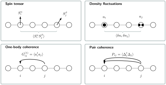
Four operator choices on the same spatial slice. Spin and density products compare local observables; $G^{(1)}_{ij}$ transfers one particle between modes in the matrix element; and $P_{ij}$ compares neutral pair amplitudes. The separation is the same geometric variable, but the operators ask different physical questions.

No operator-independent quantity deserves the name “the correlation.” Four common choices are

$$\begin{aligned} C_S^{\alpha\beta}(i,j) &= \left\langle S_i^\alpha S_j^\beta \right\rangle, \\ C_n(i,j) &= \left\langle n_i n_j \right\rangle, \\ G_{ij}^{(1)} &= \left\langle a_i^\dagger a_j \right\rangle, \\ P_{ij} &= \left\langle \Delta_i^\dagger\Delta_j \right\rangle. \end{aligned}$$

They probe, respectively, magnetic structure, occupation fluctuations, one-particle coherence, and pair coherence. Their units, symmetry properties, contact terms, and long-distance meanings differ.

Translation Symmetry and Spatial Averaging

If the state and Hamiltonian are translation invariant, then

$$C_{AB}(i,j) = C_{AB}(\mathbf r_i-\mathbf r_j).$$

On a periodic lattice, an estimator at displacement $\mathbf r$ is commonly

$$\overline C_{AB}(\mathbf r) = \frac{1}{L} \sum_i \left\langle A_i B_{i+\mathbf r} \right\rangle.$$

The addition $i+\mathbf r$ is understood modulo the periodic lattice. Averaging over origins improves statistics and enforces translation symmetry that may be weakly broken by numerical noise.

For open boundaries, only $N_{\mathbf r}$ ordered pairs have the chosen displacement:

$$\overline C_{AB}(\mathbf r) = \frac{1}{N_{\mathbf r}} \sum_{i:\,i+\mathbf r\in\Lambda} \left\langle A_i B_{i+\mathbf r} \right\rangle.$$

Using $1/L$ here creates a purely geometric decay because fewer pairs survive at large separation.

Further averaging over all displacement vectors with the same length produces a radial correlator,

$$\overline C_{AB}(r) = \frac{1}{N_r} \sum_{\lvert\mathbf r\rvert=r} \overline C_{AB}(\mathbf r).$$

This is appropriate only when rotational or point-group averaging matches the question. It can hide stripes, nematicity, bond direction, sublattice structure, and anisotropic correlation lengths.

In a trap, near an edge, or with quenched disorder, $C(i,j)$ generally contains information that $C(i-j)$ discards. One may average over a central window or disorder realizations, but that is an analysis choice, not a symmetry identity.

Raw and Connected Correlations

For the fixed operator order,

$$C_{AB}^c(i,j) = \left\langle A_i B_j \right\rangle - \left\langle A_i\right\rangle \left\langle B_j\right\rangle.$$

The raw correlator contains both mean profiles and correlated fluctuations. The connected correlator removes the product of one-point functions.

This distinction changes the asymptotic question. If a selected pure phase has

$$\left\langle O_i\right\rangle = m,$$

then its raw correlator may approach $m^2$ while its connected part approaches zero. Conversely, a finite symmetry-preserving state may have $\langle O_i\rangle=0$ while $\langle O_iO_j\rangle$ remains large over the available system. Long-Range Order gives the pointwise, volume-averaged, and structure-factor tests needed to turn that observation into a thermodynamic claim.

Subtraction can also be numerically delicate:

$$C_{AB}^c = C_{AB} - \langle A\rangle\langle B\rangle$$

may be the difference of two large estimates. A centered estimator formed from the same samples usually has better correlated-error behavior than subtracting independently rounded numbers.

Connectedness is not symmetrization and does not by itself diagnose entanglement. Those distinctions are developed in the Correlation Functions Overview.

Spin–Spin Correlations

The most informative general local object is the spin-correlation tensor

$$C_S^{\alpha\beta}(i,j) = \left\langle S_i^\alpha S_j^\beta \right\rangle.$$

Its connected version subtracts the local magnetizations:

$$C_{S,c}^{\alpha\beta}(i,j) = C_S^{\alpha\beta}(i,j) - \left\langle S_i^\alpha\right\rangle \left\langle S_j^\beta\right\rangle.$$

Contracting Cartesian components gives the rotational scalar

$$C_S(i,j) = \left\langle \mathbf S_i\cdot\mathbf S_j \right\rangle = \sum_{\alpha=x,y,z} C_S^{\alpha\alpha}(i,j).$$

If the state is invariant under global spin rotations and carries no preferred spin direction,

$$C_S^{\alpha\beta}(i,j) = \frac{\delta_{\alpha\beta}}{3} C_S(i,j).$$

This reduction fails in a magnetic field, an anisotropic Hamiltonian, a symmetry-broken state, or a spin-orbit-coupled system. Reporting only $C^{zz}$ without the symmetry assumptions can therefore miss transverse structure.

Longitudinal and transverse forms

With

$$S_i^\pm = S_i^x \pm iS_i^y,$$

one often compares

$$C^{zz}(i,j) = \left\langle S_i^zS_j^z \right\rangle$$

with

$$C^{+-}(i,j) = \left\langle S_i^+S_j^- \right\rangle.$$

The latter transfers one unit of spin projection from $j$ to $i$. It can be complex when currents, chirality, or broken time-reversal symmetry are present. For distinct sites,

$$\begin{aligned} S_i^xS_j^x + S_i^yS_j^y = \frac{1}{2} \left( S_i^+S_j^- + S_i^-S_j^+ \right). \end{aligned}$$

Onsite and staggered checks

For a site carrying a fixed spin-$s$ representation,

$$\left\langle \mathbf S_i^2 \right\rangle = \hbar^2s(s+1).$$

Any numerical tensor must reproduce this onsite sum. In a spin-$1/2$ model,

$$\left(S_i^\alpha\right)^2 = \frac{\hbar^2}{4}.$$

Antiferromagnetic correlations oscillate between sublattices. On a bipartite chain, the staggered quantity

$$C_{\mathrm{stag}}(r) = (-1)^r \left\langle \mathbf S_i\cdot\mathbf S_{i+r} \right\rangle$$

removes the leading Néel sign alternation but does not change the decay envelope. On a general lattice, the ordering wavevector or sublattice character should be stated rather than hidden in an ad hoc sign.

The Heisenberg Model owns model-specific magnetic regimes and their interpretation.

Density–Density Correlations

For lattice occupations,

$$C_n(i,j) = \left\langle n_i n_j \right\rangle, \qquad C_n^c(i,j) = \left\langle \delta n_i\delta n_j \right\rangle,$$

where

$$\delta n_i = n_i - \left\langle n_i\right\rangle.$$

The onsite connected value is the local number variance:

$$C_n^c(i,i) = \operatorname{Var}(n_i) \geq 0.$$

For a single spinless fermionic mode, $n_i^2=n_i$, so

$$\operatorname{Var}(n_i) = \left\langle n_i\right\rangle \left( 1-\left\langle n_i\right\rangle \right).$$

For bosons, $n_i^2$ is not equal to $n_i$; arbitrary occupation and bunching are possible.

Region fluctuations

For a region $A$ with

$$N_A = \sum_{i\in A}n_i,$$

the number variance is exactly

$$\operatorname{Var}(N_A) = \sum_{i,j\in A} C_n^c(i,j).$$

This identity converts a correlation map into a fluctuation of a coarse-grained observable. It also exposes the balance between positive onsite variance and offsite anticorrelation.

If the total number is sharp,

$$N = \sum_j n_j,$$

then

$$\sum_j C_n^c(i,j) = 0.$$

The positive onsite term must be compensated by correlations elsewhere unless it vanishes. This fixed-number sum rule is an exact ensemble diagnostic, not evidence of a local repulsive interaction.

Continuum contact term

For

$$n(\mathbf x) = \psi^\dagger(\mathbf x)\psi(\mathbf x),$$

the equal-time canonical algebra gives, for either statistics,

$$\begin{aligned} n(\mathbf x)n(\mathbf y) ={}& \psi^\dagger(\mathbf x) \psi^\dagger(\mathbf y) \psi(\mathbf y) \psi(\mathbf x) \\ &+ \delta^{(d)}(\mathbf x-\mathbf y) \psi^\dagger(\mathbf x) \psi(\mathbf y). \end{aligned}$$

Define the mean density by

$$\overline n(\mathbf x) = \left\langle n(\mathbf x) \right\rangle.$$

The first line of the operator identity is vacuum normal ordered. The second is the self or contact contribution. Inside an expectation value, the delta distribution samples the mean local density:

$$\delta^{(d)}(\mathbf x-\mathbf y) \left\langle \psi^\dagger(\mathbf x)\psi(\mathbf y) \right\rangle = \delta^{(d)}(\mathbf x-\mathbf y) \overline n(\mathbf x).$$

Consequently, a particle-pair counter and an ordinary product of density operators need not report the same coincident-point quantity. Normal ordering removes self-counting under the empty-vacuum convention; detector smearing turns the delta distribution into a resolution-dependent finite contribution.

Normalized pair distribution

For nonzero local densities, a common normalized second-order coherence is

$$g^{(2)}(\mathbf x,\mathbf y) = \frac{ \left\langle \psi^\dagger(\mathbf x) \psi^\dagger(\mathbf y) \psi(\mathbf y) \psi(\mathbf x) \right\rangle }{ \overline n(\mathbf x) \overline n(\mathbf y) }.$$

This definition excludes the contact self-count and is dimensionless. It becomes ill-conditioned where either density vanishes, and conventions differ for internal-state sums and detector binning.

In a number-conserving Gaussian state with no anomalous average, Wick factorization gives

$$\begin{aligned} & \left\langle \psi^\dagger(\mathbf x) \psi^\dagger(\mathbf y) \psi(\mathbf y) \psi(\mathbf x) \right\rangle \\ &\qquad= \overline n(\mathbf x) \overline n(\mathbf y) + \eta \left| G^{(1)}(\mathbf x,\mathbf y) \right|^2. \end{aligned}$$

Bosons bunch and identical fermions antibunch through the exchange term. The formula requires a Gaussian state and compatible internal labels. Interactions, fixed-number projection, anomalous contractions, and spin sums can modify it.

One-Body Density Matrix

Using the many-body convention of One-Body Operators, define

$$\gamma_{i\alpha,j\beta} = \left\langle a_{j\beta}^\dagger a_{i\alpha} \right\rangle.$$

As a matrix on the one-particle Hilbert space,

$$\gamma^\dagger = \gamma, \qquad \gamma \geq 0, \qquad \operatorname{Tr}\gamma = \langle N\rangle.$$

The frequently plotted coherence

$$G_{\alpha\beta}^{(1)}(i,j) = \left\langle a_{i\alpha}^\dagger a_{j\beta} \right\rangle$$

is the transposed-index kernel,

$$G_{\alpha\beta}^{(1)}(i,j) = \gamma_{j\beta,i\alpha}.$$

Stating the index convention avoids a common matrix-transpose error.

Positivity and the coherence bound

For any coefficients $v_{i\alpha}$,

$$\sum_{i\alpha,j\beta} v_{i\alpha}^* \gamma_{i\alpha,j\beta} v_{j\beta} = \left\langle b^\dagger b \right\rangle \geq 0,$$

where

$$b = \sum_{i\alpha} v_{i\alpha}^* a_{i\alpha}.$$

The Cauchy–Schwarz inequality therefore gives

$$\left| G_{\alpha\beta}^{(1)}(i,j) \right|^2 \leq \left\langle n_{i\alpha}\right\rangle \left\langle n_{j\beta}\right\rangle.$$

Violation of this bound signals an inconsistent normalization, a sampling error larger than quoted, or a matrix that is not a physical one-body density matrix.

Natural orbitals

Diagonalizing

$$\gamma \lvert\chi_\lambda\rangle = \nu_\lambda \lvert\chi_\lambda\rangle$$

defines natural orbitals and natural occupations. For fermions,

$$0 \leq \nu_\lambda \leq 1$$

per spin-orbital. Bosonic occupations have no Pauli upper bound. A one-body density matrix determines every one-body expectation, but not general density fluctuations, pair correlations, or the full many-body state.

For bosons, an eigenvalue scaling as $O(N)$ in a thermodynamic sequence is the basis-independent Penrose–Onsager criterion for condensation. In a homogeneous phase this may appear as off-diagonal long-range order of $G^{(1)}(\mathbf x,\mathbf y)$. The dimensional restrictions, finite-size qualifications, and distinction between condensate and superfluid fractions belong to Bose–Einstein Condensation.

For fermions, the one-body kernel can decay algebraically in a normal Fermi sea and can encode a Fermi surface without any eigenvalue exceeding one. One-particle coherence is therefore not a universal synonym for bosonic condensation.

Basis and gauge covariance

Let a unitary change of one-particle basis define new annihilation operators by

$$b_\mu = \sum_i U_{i\mu}^*a_i.$$

The one-body matrix in the new basis is then

$$\gamma^{(b)} = U^\dagger \gamma^{(a)} U.$$

Its eigenvalues and trace are basis independent; individual off-diagonal entries are not.

Under a local phase redefinition,

$$a_i \longmapsto e^{i\theta_i}a_i,$$

the coherence transforms as

$$G^{(1)}(i,j) \longmapsto e^{i(\theta_j-\theta_i)} G^{(1)}(i,j).$$

Its magnitude is invariant, while its phase must be combined with the phase convention for orbitals, Peierls links, or an interferometric reference. Closed products around loops can carry gauge-invariant phase information.

Pairing Correlations

A pair operator must specify its internal and spatial structure. An onsite spin-singlet example is

$$\Delta_i = c_{i\downarrow}c_{i\uparrow}.$$

A bond singlet can instead be written

$$\Delta_{ij}^{(s)} = \frac{1}{\sqrt{2}} \left( c_{i\downarrow}c_{j\uparrow} - c_{i\uparrow}c_{j\downarrow} \right).$$

Triplet, extended-$s$, $p$-, and $d$-wave channels require different spin tensors and form factors. A phrase such as “the pairing correlation” is incomplete until that channel is declared.

For chosen local or bond-centered pair operators, the neutral equal-time correlator is

$$P(i,j) = \left\langle \Delta_i^\dagger\Delta_j \right\rangle.$$

Under global particle-number rotations,

$$c_i \longmapsto e^{i\theta}c_i, \qquad \Delta_i \longmapsto e^{2i\theta}\Delta_i,$$

so $P(i,j)$ is invariant. By contrast, the anomalous average

$$F_i = \left\langle \Delta_i \right\rangle$$

carries number charge two and vanishes in an exact fixed-$N$ state. A vanishing anomalous average therefore does not rule out pair coherence.

The number-conserving diagnostic is a four-field expectation or, more generally, the spectrum of the two-body density matrix. Pair off-diagonal long-range order corresponds to an extensive eigenvalue in the appropriate two-particle channel. The normalization and contraction identities of that matrix are fixed in Two-Body Operators; Off-Diagonal Long-Range Order owns the macroscopic-eigenvalue criterion, pair-center limit, and finite-size scaling.

Pair correlations can be enhanced at short distance without establishing a bulk paired phase. A trustworthy claim requires:

• a specified pair form factor and symmetry channel;
• subtraction or comparison appropriate to the chosen state;
• distances large compared with microscopic pair size;
• finite-size, boundary, and dimensional analysis;
• competition with other channels;
• consistency with pair susceptibility, stiffness, or spectral evidence where relevant.

The t–J Model Preview illustrates why short-range singlet enhancement on a small cluster is not by itself evidence of superconductivity.

Exact and Gaussian Benchmarks

Simple states provide stringent checks for code and interpretation.

Product states

If the state factorizes across distinct sites,

$$\rho = \bigotimes_i\rho_i,$$

then for $i\ne j$,

$$\left\langle A_iB_j \right\rangle = \left\langle A_i\right\rangle \left\langle B_j\right\rangle,$$

and the connected intersite correlator vanishes. Onsite quantum fluctuations can remain nonzero because factorization across sites says nothing about incompatible observables on one site.

Number states

For a product of mode-number eigenstates,

$$\lvert\{n_i\}\rangle,$$

one-body coherence between distinct modes vanishes:

$$\left\langle a_i^\dagger a_j \right\rangle = 0, \qquad i\ne j.$$

For one bosonic mode with occupation $n$,

$$\left\langle a^\dagger a^\dagger aa \right\rangle = n(n-1),$$

so

$$g^{(2)}(0) = 1-\frac{1}{n}.$$

This antibunching relative to a coherent state comes from exact number preparation, not fermionic exchange.

Slater determinants

For a number-conserving spinless Slater determinant, Wick’s theorem gives

$$\left\langle n_i n_j \right\rangle_c = \delta_{ij}\gamma_{ii} - \left| \gamma_{ij} \right|^2.$$

At distinct sites,

$$\left\langle n_i n_j \right\rangle_c = - \left| \gamma_{ij} \right|^2 \leq 0.$$

This exchange hole exists without interactions. At $i=j$, the formula becomes $\gamma_{ii}(1-\gamma_{ii})$, as required by $n_i^2=n_i$.

General fermionic Gaussian states

If a fermionic Gaussian reference admits an anomalous contraction

$$F_{ij} = \left\langle c_i c_j \right\rangle,$$

then

$$\left\langle n_i n_j \right\rangle_c = \delta_{ij}\gamma_{ii} - \left| \gamma_{ij} \right|^2 + \left| F_{ij} \right|^2$$

for a single-component notation with consistent indices. The exchange and pairing terms enter with opposite signs. This is a Gaussian identity, not a definition and not a valid closure for an arbitrary interacting state.

Symmetry Constraints

Symmetries reduce the number of independent entries and provide exact zero tests.

Translation and point-group symmetry

Translation invariance reduces two site labels to a displacement. Point-group operations relate symmetry-equivalent directions:

$$C(R\mathbf r) = C(\mathbf r)$$

when both the state and the transformed operator channel are invariant under $R$. Tensor and bond operators may acquire component rotations or signs, so a scalar-looking average should not be imposed before checking the representation.

Particle-number symmetry

If

$$[\rho,N] = 0,$$

then any operator $O_q$ with nonzero number charge,

$$[N,O_q] = qO_q,$$

has

$$\left\langle O_q\right\rangle = 0.$$

Neutral products such as $a_i^\dagger a_j$ and $\Delta_i^\dagger\Delta_j$ can remain nonzero.

Spin symmetry

In an $SU(2)$-invariant singlet,

$$\left\langle S_i^\alpha \right\rangle = 0$$

and the two-point tensor is isotropic. With only $U(1)$ symmetry about $z$, longitudinal and transverse correlators need not agree, but correlators carrying nonzero total $S^z$ charge vanish.

Hermiticity and exchange

For arbitrary operators,

$$C_{AB}(i,j)^* = C_{B^\dagger A^\dagger}(j,i).$$

For a one-body kernel,

$$G^{(1)}(i,j)^* = G^{(1)}(j,i).$$

For identical Hermitian observables on commuting sites,

$$C_{AA}(i,j) = C_{AA}(j,i) \in \mathbb R.$$

These relations should be checked before symmetrizing numerical data; premature symmetrization can conceal an implementation error or erase a physical chiral component.

Relation to Momentum-Space Data

Equal-time real-space data and momentum-space static data contain the same information when every separation and normalization is retained. For a periodic translation-invariant lattice, one common transform is

$$C_{AB}(\mathbf q) = \sum_{\mathbf r} e^{-i\mathbf q\cdot\mathbf r} C_{AB}(\mathbf r).$$

The inverse then carries $1/L$:

$$C_{AB}(\mathbf r) = \frac{1}{L} \sum_{\mathbf q} e^{i\mathbf q\cdot\mathbf r} C_{AB}(\mathbf q).$$

Other conventions distribute factors of $L$, volume, or $2\pi$ differently.

The momentum occupation of a lattice field is

$$n(\mathbf k) = \frac{1}{L} \sum_{i,j} e^{i\mathbf k\cdot(\mathbf r_i-\mathbf r_j)} \left\langle a_i^\dagger a_j \right\rangle.$$

Thus momentum occupation is the Fourier transform of one-body coherence, not of density–density correlations.

By contrast, a static density or spin structure factor Fourier transforms the corresponding two-observable correlator. Whether it uses the raw or connected form and whether it is divided by $L$ or $N$ must be stated.

With a compatible convention, integrating a dynamic structure factor over frequency recovers its equal-time static correlator. This statement is exact, but factors of $2\pi$ depend on the Fourier definition. Equal-time data contain total spectral weight, not the energy distribution of that weight.

Structure Factors gives the canonical normalization, zeroth-moment identity, elastic subtraction, and experimental forward models.

What Experiments Actually Estimate

Different probes access different operator orderings and resolution kernels.

Site-resolved snapshots

A projective image in an occupation basis produces samples $n_i^{(m)}$, or spin-resolved samples after suitable state mapping. Repeated shots estimate

$$\left\langle n_i n_j \right\rangle \approx \frac{1}{M} \sum_{m=1}^{M} n_i^{(m)}n_j^{(m)}.$$

The measured observable may be parity rather than occupation, may merge internal states, and may include loss or misclassification. Detection fidelity must be folded into the estimator or corrected with a calibrated response model.

Transverse spin correlations usually require a controlled spin rotation before measurement in the laboratory quantization basis. The rotation is part of the measurement definition.

Scattering

Elastic and energy-integrated scattering intensities are related to spatial Fourier transforms of density or spin correlations, multiplied by form factors, polarization factors, and instrumental resolution. A measured intensity is not a bare structure factor until those ingredients and disconnected elastic contributions are handled.

Interference and expansion

Time-of-flight or interference measurements can access momentum occupation and therefore one-body coherence, but the image also contains Wannier envelopes, finite expansion effects, interactions during expansion, and line-of-sight integration.

Noise correlations of expanded density can reveal two-body and pairing information. They estimate a density–density object after a nontrivial mapping from in-trap modes to detector coordinates; they do not turn a four-field correlator into a one-body expectation.

Pair-sensitive probes

Pair transfer, molecule conversion, Josephson interference, and two-particle noise can be sensitive to pair channels. Each introduces a form factor and often a dynamical protocol. An equal-time pair correlator is the theoretical target only after the measurement map is established.

Computation and Estimation

Exact diagonalization

For a state vector,

$$C_{AB}(i,j) = \langle\Psi\rvert A_iB_j \lvert\Psi\rangle.$$

Apply the rightmost operator first. For fermionic operators, a basis-state implementation must preserve the global mode ordering and its parity signs. Exact onsite identities, Hermiticity, and conserved-number sum rules are inexpensive tests.

Tensor networks

Matrix-product states and projected entangled-pair states evaluate local and string correlators by tensor contraction. Long-distance connected correlators can be much smaller than the raw terms, so contraction accuracy and subtraction error must be monitored. In one dimension, transfer-matrix eigenvalues organize asymptotic decay, but finite bond dimension can impose an artificial correlation length.

Quantum Monte Carlo

Equal-time diagonal observables may admit direct estimators, whereas off-diagonal coherence and pair operators can require improved or worm estimators. Statistical uncertainty grows when subtracting disconnected pieces, and Markov-chain autocorrelation reduces the effective number of independent samples.

Sign-problem-free sampling is model and basis dependent. A small error bar within a biased or constrained ensemble does not establish correctness for the intended Hamiltonian.

Experimental or synthetic samples

For independent scalar samples $(a_m,b_m)$, the unbiased sample covariance is

$$\widehat C_{AB}^c = \frac{1}{M-1} \sum_{m=1}^{M} \left( a_m-\overline a \right) \left( b_m-\overline b \right).$$

For correlated time-series or Markov-chain data, $M$ must be replaced conceptually by an effective sample size obtained from autocorrelation analysis. Spatially averaging many pairs in one snapshot also does not make those pairs statistically independent.

Finite-Size and Boundary Audits

Before interpreting a spatial correlation curve:

1. State open, periodic, twisted, trapped, or disordered boundary conditions.
2. Distinguish the displacement vector $\mathbf r$ from its shortest periodic representative.
3. Record the number of contributing pairs at each separation.
4. Keep sublattice, bond, orbital, and tensor labels until symmetry justifies averaging.
5. Separate lattice-scale contact behavior from asymptotic behavior.
6. Compare distances with both microscopic scales and the system size.
7. Repeat at several sizes before claiming a plateau or a decay exponent.
8. Check whether a fixed global charge forces a compensating long-range anticorrelation.
9. Propagate covariance among raw, mean, and connected estimates.
10. Test exact onsite and sum-rule identities.

On a periodic chain, separations $r$ and $L-r$ refer to the same shortest geometric distance but can correspond to opposite directed displacements for complex correlators. Folding the data is justified only after verifying the relevant conjugation or inversion relation.

Common Mistakes

• Calling an equal-time correlator time independent without checking stationarity.
• Assuming equal-time Hermitian products are automatically real.
• Changing operator order at coincident sites.
• Using one symbol for raw, connected, symmetrized, and normal-ordered correlations.
• Treating $\mathbf x=\mathbf y$ in a continuum formula without contact terms or smearing.
• Confusing momentum occupation with a density structure factor.
• Interpreting every off-diagonal one-body matrix element as a basis-independent observable.
• Inferring bosonic condensation from one finite-system matrix element instead of the spectrum and scaling of $\gamma$.
• Inferring superconductivity from a large nearest-neighbor pair correlator on one cluster.
• Applying Wick factorization to an arbitrary interacting state.
• Calling a fixed-number anticorrelation direct evidence of repulsion.
• Dividing an open-boundary displacement average by $L$ rather than by the number of valid pairs.
• Radially averaging before checking anisotropy or ordering wavevectors.
• Ignoring detector parity projection, point-spread functions, or internal-state resolution.
• Treating all measured pairs in one image as statistically independent.
• Enforcing a symmetry on numerical data before using that symmetry as a validation test.

Reliable Workflow

1. Name the state or ensemble and decide whether it is stationary.
2. Write the operators with all spatial, internal, and bond labels.
3. Fix their literal order and say whether normal ordering is applied.
4. Decide whether the physical question concerns raw or connected data.
5. State lattice, continuum, smearing, and cell-volume conventions.
6. Use symmetry only after checking how the operator channel transforms.
7. Audit onsite algebra, Hermiticity, positivity, and conserved-charge sums.
8. Preserve directional data before optional spatial averaging.
9. Map the theoretical correlator through the actual measurement or numerical estimator.
10. Establish size, resolution, sampling, and asymptotic convergence before assigning a phase.

Exercises

Exercise 1: Common-time invariance

Let

$$C_{AB}(t) = \operatorname{Tr} \left[ \rho A_H(t)B_H(t) \right].$$

Show that $dC_{AB}/dt=0$ when $[H,\rho]=0$. Give one reason this result can fail.

Solution

Because both operators carry the same time,

$$A_H(t)B_H(t) = e^{iHt/\hbar} AB e^{-iHt/\hbar}.$$

Differentiation gives

$$\frac{dC_{AB}}{dt} = \frac{i}{\hbar} \operatorname{Tr} \left( \rho [H,A_H(t)B_H(t)] \right).$$

Using cyclicity,

$$\begin{aligned} \operatorname{Tr} \left( \rho[H,X] \right) &= \operatorname{Tr} \left( \rho HX-\rho XH \right) \\ &= \operatorname{Tr} \left( X\rho H-XH\rho \right) \\ &= \operatorname{Tr} \left( X[\rho,H] \right) = 0. \end{aligned}$$

The result can fail after a quench when $\rho$ does not commute with the post-quench Hamiltonian, under explicit time-dependent driving, or when the measured operators themselves have explicit time dependence beyond Heisenberg evolution.

Exercise 2: Ordered spin products

For a spin-$1/2$ in the state $\lvert\uparrow_z\rangle$, evaluate

$$\left\langle S^xS^y \right\rangle, \qquad \left\langle S^yS^x \right\rangle,$$

and their symmetrized average.

Solution

Using $S^\alpha=\hbar\sigma_\alpha/2$ and

$$\sigma_x\sigma_y = i\sigma_z, \qquad \sigma_y\sigma_x = -i\sigma_z,$$

we find

$$\left\langle S^xS^y \right\rangle = \frac{i\hbar^2}{4},$$

and

$$\left\langle S^yS^x \right\rangle = -\frac{i\hbar^2}{4}.$$

Therefore

$$\frac{1}{2} \left\langle \{S^x,S^y\} \right\rangle = 0.$$

The equal-time ordered products are complex conjugates, while the symmetrized correlation is real. Equal time did not make the two operators commute.

Exercise 3: Fixed-number sum rule

Suppose $N=\sum_jn_j$ has exactly the value $N_0$. Prove that

$$\sum_j \left\langle \delta n_i\delta n_j \right\rangle = 0.$$

Explain the consequence when $\operatorname{Var}(n_i)>0$.

Solution

Because the total number has no fluctuation,

$$\delta N = N-\langle N\rangle = \sum_j\delta n_j = 0$$

on the support of the state. Hence

$$\begin{aligned} \sum_j \left\langle \delta n_i\delta n_j \right\rangle &= \left\langle \delta n_i \sum_j\delta n_j \right\rangle \\ &= \left\langle \delta n_i\delta N \right\rangle = 0. \end{aligned}$$

The $j=i$ contribution is

$$\left\langle (\delta n_i)^2 \right\rangle = \operatorname{Var}(n_i) \geq 0.$$

If it is strictly positive, the sum of offsite connected correlations must be negative. The compensation follows from the global constraint even in a noninteracting system.

Exercise 4: Exchange hole of a Slater determinant

For a spinless, number-conserving Slater determinant, let

$$\gamma_{ij} = \left\langle c_j^\dagger c_i \right\rangle.$$

Use Wick’s theorem to show

$$\left\langle n_i n_j \right\rangle_c = \delta_{ij}\gamma_{ii} - \left| \gamma_{ij} \right|^2.$$

Solution

Start from

$$n_i n_j = c_i^\dagger c_i c_j^\dagger c_j.$$

The canonical anticommutator gives

$$c_i c_j^\dagger = \delta_{ij} - c_j^\dagger c_i,$$

so

$$n_i n_j = \delta_{ij}c_i^\dagger c_j + c_i^\dagger c_j^\dagger c_j c_i.$$

For a number-conserving Slater determinant,

$$\left\langle c_i^\dagger c_j^\dagger c_j c_i \right\rangle = \gamma_{ii}\gamma_{jj} - \gamma_{ij}\gamma_{ji}.$$

Hermiticity gives $\gamma_{ji}=\gamma_{ij}^*$. Subtracting

$$\langle n_i\rangle \langle n_j\rangle = \gamma_{ii}\gamma_{jj}$$

yields

$$\left\langle n_i n_j \right\rangle_c = \delta_{ij}\gamma_{ii} - \left| \gamma_{ij} \right|^2.$$

At $i\ne j$, the result is nonpositive and represents Pauli exchange rather than dynamical repulsion.

Exercise 5: Positivity bound for one-body coherence

Prove

$$\left| \left\langle a_i^\dagger a_j \right\rangle \right|^2 \leq \left\langle n_i\right\rangle \left\langle n_j\right\rangle$$

for either bosons or fermions.

Solution

Define an inner product on operators by

$$(X,Y)_\rho = \left\langle X^\dagger Y \right\rangle_\rho.$$

It is positive semidefinite because

$$(X,X)_\rho = \left\langle X^\dagger X \right\rangle_\rho \geq 0.$$

Cauchy–Schwarz with $X=a_i$ and $Y=a_j$ gives

$$\left| \left\langle a_i^\dagger a_j \right\rangle \right|^2 \leq \left\langle a_i^\dagger a_i \right\rangle \left\langle a_j^\dagger a_j \right\rangle.$$

The right-hand side is $\langle n_i\rangle\langle n_j\rangle$. No assumption about Gaussianity, particle statistics, or stationarity was needed.

Exercise 6: Number-state second-order coherence

For a bosonic number state $\lvert n\rangle$, calculate

$$g^{(2)}(0) = \frac{ \langle a^\dagger a^\dagger aa \rangle }{ \langle a^\dagger a\rangle^2 }.$$

Compare $n=1$ with the large-$n$ limit.

Solution

The ladder relations give

$$aa\lvert n\rangle = \sqrt{n(n-1)} \lvert n-2\rangle.$$

Therefore

$$\left\langle a^\dagger a^\dagger aa \right\rangle = n(n-1),$$

while

$$\left\langle a^\dagger a \right\rangle = n.$$

For $n>0$,

$$g^{(2)}(0) = \frac{n(n-1)}{n^2} = 1-\frac{1}{n}.$$

A one-boson number state has $g^{(2)}(0)=0$ because it cannot provide a detected pair. As $n\to\infty$, $g^{(2)}(0)\to1$, although the state remains a number state rather than a coherent state. This one normalized moment does not reconstruct the state.

Exercise 7: Number symmetry and pair coherence

Let $\lvert\Psi_N\rangle$ have sharp particle number $N$. Show that

$$\left\langle \Psi_N \middle| \Delta_i \middle| \Psi_N \right\rangle = 0$$

for a pair annihilation operator satisfying $[N,\Delta_i]=-2\Delta_i$. Why can

$$\left\langle \Delta_i^\dagger\Delta_j \right\rangle$$

remain nonzero?

Solution

The commutator implies

$$N\Delta_i\lvert\Psi_N\rangle = (N-2) \Delta_i\lvert\Psi_N\rangle.$$

Thus $\Delta_i\lvert\Psi_N\rangle$ lies in the $(N-2)$-particle sector, which is orthogonal to $\lvert\Psi_N\rangle$. Their overlap vanishes.

The product $\Delta_i^\dagger\Delta_j$ removes two particles and then restores two. It has zero total number charge:

$$[N,\Delta_i^\dagger\Delta_j] = 0.$$

Its expectation can therefore be nonzero in a fixed-$N$ state and can diagnose pair coherence without introducing a number-breaking anomalous mean.

Exercise 8: Open-chain displacement average

An open chain has $L$ sites. For a positive displacement $r<L$, how many ordered pairs $(i,i+r)$ exist? Write the unbiased geometric average of $\langle A_iB_{i+r}\rangle$. What spurious factor appears if one divides by $L$ instead?

Solution

The allowed origins are

$$i = 1,2,\ldots,L-r,$$

so

$$N_r = L-r.$$

The displacement average is

$$\overline C_{AB}(r) = \frac{1}{L-r} \sum_{i=1}^{L-r} \left\langle A_iB_{i+r} \right\rangle.$$

If every pair expectation equals a constant $C_0$, this estimator returns $C_0$. Dividing by $L$ instead gives

$$\frac{1}{L} \sum_{i=1}^{L-r}C_0 = \left( 1-\frac{r}{L} \right) C_0.$$

The apparent linear decay is a boundary pair-counting artifact.

Cross-Links

• Correlation Function Definitions — canonical notation for equal-time, connected, and structure-factor objects.
• Correlation Functions Overview — hierarchy, connectedness, decay, ordering prescriptions, and static-versus-dynamic map.
• Time-Dependent Correlations — unequal-time ordering, Lehmann spectra, dephasing, and recurrence.
• Structure Factors — momentum-space transforms and scattering observables.
• Correlation Functions Formula Card — compact lookup conventions.
• One-Body Operators — one-body reduced density matrices, natural orbitals, and expectation values.
• Two-Body Operators — two-body reduced density matrices, contractions, and pair normalization.
• Real-Space Representation — continuum-to-lattice normalization and cell averages.
• Normal Ordering in Many-Body QM — contact terms, reference contractions, and anomalous averages.
• Occupation Numbers — natural occupations and ensemble-dependent number fluctuations.
• Bose–Einstein Condensation — macroscopic one-body eigenvalues and off-diagonal long-range order.
• Density Operators and Current Operators — local densities, currents, and continuity equations.
• Heisenberg Model — magnetic correlation patterns in exchange models.
• Hubbard Model — spin, charge, one-body, and double-occupancy observables.
• Bose–Hubbard Model — coherence, number fluctuations, and Mott versus superfluid tendencies.
• t–J Model Preview — projected spin, charge, and singlet-pair correlators.
• Kubo Formula — why retarded response uses a causal commutator rather than an ordinary equal-time product.

References

1. A. L. Fetter and J. D. Walecka, Quantum Theory of Many-Particle Systems, Dover (2003).
2. J. W. Negele and H. Orland, Quantum Many-Particle Systems, Westview Press (1998).
3. G. D. Mahan, Many-Particle Physics, 3rd ed., Springer (2000).
4. P. Coleman, Introduction to Many-Body Physics, Cambridge University Press (2015).
5. A. Altland and B. Simons, Condensed Matter Field Theory, 2nd ed., Cambridge University Press (2010).
6. A. Auerbach, Interacting Electrons and Quantum Magnetism, Springer (1994).
7. P.-O. Löwdin, “Quantum Theory of Many-Particle Systems. I. Physical Interpretations by Means of Density Matrices, Natural Spin-Orbitals, and Convergence Problems in the Method of Configurational Interaction”, Physical Review 97, 1474–1489 (1955).
8. O. Penrose and L. Onsager, “Bose–Einstein Condensation and Liquid Helium”, Physical Review 104, 576–584 (1956).
9. C. N. Yang, “Concept of Off-Diagonal Long-Range Order and the Quantum Phases of Liquid He and of Superconductors”, Reviews of Modern Physics 34, 694–704 (1962).
10. A. J. Coleman, “Structure of Fermion Density Matrices”, Reviews of Modern Physics 35, 668–686 (1963).
11. G. C. Wick, “The Evaluation of the Collision Matrix”, Physical Review 80, 268–272 (1950).
12. R. J. Glauber, “The Quantum Theory of Optical Coherence”, Physical Review 130, 2529–2539 (1963).
13. E. Altman, E. Demler, and M. D. Lukin, “Probing Many-Body States of Ultracold Atoms via Noise Correlations”, Physical Review A 70, 013603 (2004).
14. L. W. Cheuk, M. A. Nichols, M. Okan, T. Gersdorf, V. V. Ramasesh, W. S. Bakr, T. Lompe, and M. W. Zwierlein, “Quantum-Gas Microscope for Fermionic Atoms”, Physical Review Letters 114, 193001 (2015).