Density Operators and Current Operators

A density operator says where an extensive quantity is stored. A current operator says how that quantity crosses space or lattice bonds. Their relation is a local conservation law: a region can lose particle number, charge, or another conserved quantity only through outward flux, unless the effective dynamics contains an explicit source or sink.

For one nonrelativistic field, the central operators are

$$\begin{aligned} n(\mathbf r) &= \psi^\dagger(\mathbf r) \psi(\mathbf r), \\ \mathbf j_N(\mathbf r) &= \frac{\hbar}{2mi} \left[ \psi^\dagger\nabla\psi - (\nabla\psi^\dagger)\psi \right], \end{aligned}$$

and, for a number-conserving Schrödinger Hamiltonian,

$$\frac{\partial n}{\partial t} + \nabla\boldsymbol\cdot\mathbf j_N = 0.$$

These are operator identities. Taking expectation values gives the measurable mean density and mean current, but does not replace the operators or determine their fluctuations.

This page is the canonical home for many-body density and current operators. Probability Current owns the one-particle wave-mechanics formula, and Field Operators in Many-Body Models owns the field construction. Kubo Formula owns the source-response derivation and conductivity contact terms; Transport Coefficients Preview owns the coefficient and hydrodynamic-limit dictionary. Hydrodynamics and Effective Theory Preview owns the long-wavelength field content, constitutive expansion, fluctuations, and effective-theory handoff. Collective Modes owns how continuity equations combine with constitutive or inertial dynamics to produce diffusion, sound, and coupled response eigenmodes. Plasmons Preview applies the number and charge continuity equations to self-consistent longitudinal electric fields.

Superfluidity in Condensed Matter applies these number, mass-density, and current conventions to neutral two-fluid response; this page retains the operator definitions and continuity identities.

Conventions

Unless stated otherwise:

• fields are evaluated at equal time;
• $\mathbf r$ is a point in $d$ spatial dimensions;
• $\alpha,\beta$ label internal components such as spin;
• repeated internal labels are summed only when a sum is displayed;
• $n$ denotes number density, not a density matrix;
• $\mathbf j_N$ denotes particle-number current;
• $\mathbf j_q$ denotes electric-charge current;
• an outward current from site $i$ to site $j$ is positive as $I_{i\to j}$;
• the fields may be bosonic or fermionic, with their appropriate equal-time algebra.

The visible bilinear formulas for density and current are often identical for bosons and fermions. Statistics enters through the field algebra, allowed states, and correlation functions.

Local Number Density

For one field species,

$$n(\mathbf r) = \psi^\dagger(\mathbf r) \psi(\mathbf r).$$

For several internal components,

$$n(\mathbf r) = \sum_\alpha \psi_\alpha^\dagger(\mathbf r) \psi_\alpha(\mathbf r).$$

The total number operator is

$$N = \int d^dr\, n(\mathbf r).$$

For a normalized state $\lvert\Psi\rangle$,

$$\langle n(\mathbf r)\rangle = \langle\Psi\vert n(\mathbf r) \vert\Psi\rangle$$

is the expected number per unit volume near $\mathbf r$. In a fixed-$N$ sector,

$$\int d^dr\, \langle n(\mathbf r)\rangle = N.$$

This is not generally a probability density normalized to one. The normalized one-particle spatial marginal is $\langle n(\mathbf r)\rangle/N$ when $N>0$ is fixed.

Smeared Densities and Regions

Continuum fields are operator-valued distributions, so a mathematically safer object is a smeared density

$$N_f = \int d^dr\, f(\mathbf r)n(\mathbf r),$$

where $f$ is a suitable test function. If $f\ge0$, then $N_f$ is positive on its natural domain.

For a spatial region $\Omega$, choose the indicator function of the region:

$$N_\Omega = \int_\Omega d^dr\, n(\mathbf r).$$

This operator counts particles in $\Omega$. Its expectation need not be an integer because a quantum state can have number fluctuations in the region even when total $N$ is sharp.

The density generates local phase rotations through

$$\begin{aligned} [n(\mathbf r),\psi(\mathbf r')] &= -\delta^{(d)}(\mathbf r-\mathbf r') \psi(\mathbf r'), \\ [n(\mathbf r),\psi^\dagger(\mathbf r')] &= \delta^{(d)}(\mathbf r-\mathbf r') \psi^\dagger(\mathbf r'). \end{aligned}$$

These are ordinary commutators because the density is an even operator for either statistics.

Density in a Mode Basis

Expand the field in orthonormal one-particle modes:

$$\psi(x) = \sum_i \varphi_i(x)a_i,$$

where $x$ may include position and an internal label. The local density becomes

$$n(x) = \sum_{i,j} \varphi_i^*(x) \varphi_j(x) a_i^\dagger a_j.$$

The diagonal terms contain mode occupations. The off-diagonal terms contain one-body coherences and can produce spatial interference. A density profile is therefore not determined by occupation numbers alone unless the one-body density matrix is diagonal in the chosen basis.

Completeness gives

$$\begin{aligned} \int dx\,n(x) &= \sum_{i,j} a_i^\dagger a_j \int dx\, \varphi_i^*(x)\varphi_j(x), \\ &= \sum_i a_i^\dagger a_i = N. \end{aligned}$$

This is a concrete example of the general lift derived in One-Body Operators. Its evaluation from one-body density matrices is developed in the many-body application guide.

Relation to First Quantization

Let $\Psi_N(x_1,\ldots,x_N)$ be a normalized symmetric or antisymmetric wavefunction. Then

$$\begin{aligned} \langle n(x)\rangle ={}& N \int dx_2\cdots dx_N \\ &\times \left| \Psi_N(x,x_2,\ldots,x_N) \right|^2. \end{aligned}$$

The factor $N$ appears because any one of the $N$ identical particles can occupy the observed coordinate. Integrating over $x$ returns $N$.

For spinless particles, the corresponding number-current expectation is

$$\begin{aligned} \langle\mathbf j_N(\mathbf r)\rangle ={}& \frac{N\hbar}{2mi} \int dx_2\cdots dx_N \\ &\times \left[ \Psi_N^*\nabla_{\mathbf r}\Psi_N - (\nabla_{\mathbf r}\Psi_N^*)\Psi_N \right], \end{aligned}$$

where the first coordinate has position $\mathbf r$ and the remaining coordinates are integrated. Internal labels are summed when present. For $N=1$, this reduces to the ordinary probability current.

Charge, Mass, and Species Densities

For particles of charge $q$ and mass $m$,

$$\rho_q(\mathbf r) = q\,n(\mathbf r), \qquad \rho_m(\mathbf r) = m\,n(\mathbf r).$$

For several species $s$,

$$\rho_q = \sum_s q_s n_s, \qquad \rho_m = \sum_s m_s n_s.$$

A species number $N_s$ is conserved only if the Hamiltonian does not convert that species into another. Total electric charge may remain conserved even when individual species populations change.

The corresponding currents are weighted in the same way:

$$\mathbf j_q = \sum_s q_s\mathbf j_{N,s}, \qquad \mathbf j_m = \sum_s m_s\mathbf j_{N,s}.$$

Number current, charge current, and mass current have different units and should not be denoted by the same symbol without a stated convention.

Spin Density

For a two-component spinor field

$$\psi = \begin{pmatrix} \psi_\uparrow\\ \psi_\downarrow \end{pmatrix},$$

the physical spin-angular-momentum density is

$$s^a(\mathbf r) = \frac{\hbar}{2} \psi^\dagger(\mathbf r) \sigma^a \psi(\mathbf r),$$

where $\sigma^a$ is a Pauli matrix. In particular,

$$\begin{aligned} s^z &= \frac{\hbar}{2} \left( n_\uparrow-n_\downarrow \right), \\ n &= n_\uparrow+n_\downarrow. \end{aligned}$$

The transverse components depend on spin coherence:

$$\begin{aligned} s^x &= \frac{\hbar}{2} \left( \psi_\uparrow^\dagger\psi_\downarrow + \psi_\downarrow^\dagger\psi_\uparrow \right), \\ s^y &= \frac{\hbar}{2i} \left( \psi_\uparrow^\dagger\psi_\downarrow - \psi_\downarrow^\dagger\psi_\uparrow \right). \end{aligned}$$

Thus the pair of component densities $n_\uparrow,n_\downarrow$ determines $s^z$ but not the full spin vector.

The Kondo Model Preview couples a localized spin to this conduction spin density at one position. Its exchange transfers spin while preserving the total spin of impurity plus bath.

Continuum Number Current

Consider a spin-independent Schrödinger Hamiltonian

$$\begin{aligned} H_0 = \sum_\alpha \int d^dr\, \biggl[ & \frac{\hbar^2}{2m} \nabla\psi_\alpha^\dagger \boldsymbol\cdot \nabla\psi_\alpha \\ &+ U(\mathbf r) \psi_\alpha^\dagger\psi_\alpha \biggr]. \end{aligned}$$

The particle-number current is

$$\begin{aligned} \mathbf j_N(\mathbf r) = \frac{\hbar}{2mi} \sum_\alpha \bigl[ & \psi_\alpha^\dagger \nabla\psi_\alpha \\ &- (\nabla\psi_\alpha^\dagger) \psi_\alpha \bigr]. \end{aligned}$$

It is Hermitian. An equivalent symmetrized-velocity form is

$$\begin{aligned} \mathbf j_N = \frac1{2m} \sum_\alpha \bigl[ & \psi_\alpha^\dagger (-i\hbar\nabla)\psi_\alpha \\ &+ \bigl((-i\hbar\nabla)\psi_\alpha\bigr)^\dagger \psi_\alpha \bigr]. \end{aligned}$$

The expression is the same for bosonic and fermionic Schrödinger fields. It depends on the kinetic operator: a Hamiltonian with higher derivatives, nonlocal hopping, or spin-orbit coupling can require additional current terms.

Deriving the Continuity Equation

In the Heisenberg picture,

$$\frac{\partial n(\mathbf r,t)}{\partial t} = \frac{i}{\hbar} [H,n(\mathbf r,t)].$$

For the scalar one-body Hamiltonian, the field equations give

$$\begin{aligned} i\hbar\partial_t\psi &= \left( -\frac{\hbar^2}{2m}\nabla^2 + U \right)\psi, \\ -i\hbar\partial_t\psi^\dagger &= -\frac{\hbar^2}{2m}\nabla^2\psi^\dagger + U\psi^\dagger. \end{aligned}$$

Differentiate $n=\psi^\dagger\psi$:

$$\begin{aligned} \partial_t n &= (\partial_t\psi^\dagger)\psi + \psi^\dagger(\partial_t\psi), \\ &= \frac{i\hbar}{2m} \left[ \psi^\dagger\nabla^2\psi - (\nabla^2\psi^\dagger)\psi \right]. \end{aligned}$$

The scalar potential cancels. Using

$$\begin{aligned} \nabla\boldsymbol\cdot \left[ \psi^\dagger\nabla\psi - (\nabla\psi^\dagger)\psi \right] = & \psi^\dagger\nabla^2\psi \\ &- (\nabla^2\psi^\dagger)\psi \end{aligned}$$

produces the operator continuity equation

$$\frac{\partial n}{\partial t} + \nabla\boldsymbol\cdot\mathbf j_N = 0.$$

No expectation value or mean-field approximation was used.

What Interactions Do

A coordinate-diagonal, number-conserving pair interaction has the form

$$\begin{aligned} H_{\mathrm{int}} = \frac12 \int d^dr\,d^dr'\, & \psi^\dagger(\mathbf r) \psi^\dagger(\mathbf r') \\ &\times v(\mathbf r,\mathbf r') \psi(\mathbf r') \psi(\mathbf r). \end{aligned}$$

For such an interaction,

$$[H_{\mathrm{int}},n(\mathbf r)] = 0.$$

It changes correlations and the state that carries current, but it does not add a source to the local number equation. Density-density lattice interactions behave similarly.

This statement has boundaries. Derivative interactions can contribute to the current. Pairing terms do not conserve particle number. A nonlocal one-body kernel can transfer density without admitting the simple gradient current above. The current must be derived from the actual Hamiltonian rather than imported from a nearby model.

Integral Conservation Law

Integrating the continuity equation over a fixed region $\Omega$ gives

$$\frac{dN_\Omega}{dt} = - \int_\Omega d^dr\, \nabla\boldsymbol\cdot\mathbf j_N.$$

The divergence theorem yields

$$\frac{dN_\Omega}{dt} = - \oint_{\partial\Omega} \mathbf j_N \boldsymbol\cdot d\mathbf S.$$

Positive outward flux lowers the number in the region. Taking an expectation value gives the same equation for $\langle N_\Omega\rangle$ and $\langle\mathbf j_N\rangle$.

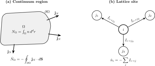
Local conservation has the same bookkeeping structure in continuum and lattice descriptions. A continuum region loses number through outward surface flux, while a lattice site loses number through the sum of oriented bond currents. A source term would appear on the right side of either equation.

For all space, total number is conserved when the boundary flux vanishes. On a periodic domain, current leaving one boundary re-enters through the identified boundary. On an open domain, the boundary condition is part of the conservation statement.

Gauge-Covariant Charge Current

For a field of charge $q$ coupled minimally to electromagnetic potentials,

$$\boldsymbol\Pi = -i\hbar\nabla-q\mathbf A,$$

and

$$H_0 = \int d^dr\, \psi^\dagger \left[ \frac{\boldsymbol\Pi^2}{2m} + q\phi \right] \psi.$$

The gauge-covariant number current is

$$\mathbf j_N = \frac1{2m} \left[ \psi^\dagger\boldsymbol\Pi\psi + (\boldsymbol\Pi\psi)^\dagger\psi \right].$$

Expanding it gives

$$\mathbf j_N = \mathbf j_{\mathrm p} - \frac{q}{m} \mathbf A\,n,$$

where

$$\mathbf j_{\mathrm p} = \frac{\hbar}{2mi} \left[ \psi^\dagger\nabla\psi - (\nabla\psi^\dagger)\psi \right]$$

is often called the paramagnetic number current. The $\mathbf A$ term is the diamagnetic contribution.

The electric-charge current is

$$\mathbf j_q = q\,\mathbf j_N.$$

Under

$$\begin{aligned} \psi &\longmapsto e^{iq\chi/\hbar}\psi, \\ \mathbf A &\longmapsto \mathbf A+\nabla\chi, \\ \phi &\longmapsto \phi-\partial_t\chi, \end{aligned}$$

the two pieces of $\mathbf j_N$ change, but their sum is invariant. The paramagnetic-diamagnetic split is convention useful; the physical current is the full gauge-covariant operator.

Equivalently, the charge current is obtained by coupling the Hamiltonian to $\mathbf A$:

$$\mathbf j_q(\mathbf r) = - \frac{\delta H}{\delta\mathbf A(\mathbf r)}.$$

This functional-derivative definition is especially useful when the kinetic operator is more complicated than $\mathbf p^2/(2m)$.

Plane Waves and Standing Waves

In a periodic volume $V$, let

$$\varphi_{\mathbf k}(\mathbf r) = \frac1{\sqrt V} e^{i\mathbf k\cdot\mathbf r}.$$

For a state with occupation $N_{\mathbf k}$ in this mode,

$$\begin{aligned} \langle n(\mathbf r)\rangle &= \frac{N_{\mathbf k}}{V}, \\ \langle\mathbf j_N(\mathbf r)\rangle &= \frac{\hbar\mathbf k}{m} \frac{N_{\mathbf k}}{V}. \end{aligned}$$

For a fermionic complete mode, $N_{\mathbf k}$ is $0$ or $1$; degeneracy can supply additional occupied modes with the same momentum.

A real standing-wave orbital has zero current even when its density varies in space. Conversely, a stationary density need not imply zero current: a momentum eigenstate on a ring has time-independent density and nonzero circulating current.

Lattice Density Operators

For a lattice mode $i$,

$$n_i = a_i^\dagger a_i.$$

For a spinful lattice site,

$$n_i = \sum_\sigma c_{i\sigma}^\dagger c_{i\sigma}.$$

The site density is dimensionless: it counts occupation of the local mode or site. A physical density per volume requires division by a cell volume or reconstruction from localized orbitals.

For a general one-body lattice Hamiltonian,

$$H_1 = \sum_{i,j} h_{ij} a_i^\dagger a_j, \qquad h_{ji}=h_{ij}^*,$$

the identity

$$[n_i,a_j^\dagger a_k] = \left( \delta_{ij}-\delta_{ik} \right) a_j^\dagger a_k$$

holds for bosons and fermions.

Oriented Bond Current

For $i\ne j$, define the particle current from $i$ to $j$ by

$$I_{i\to j} = \frac{i}{\hbar} \left( h_{ij}a_i^\dagger a_j - h_{ji}a_j^\dagger a_i \right).$$

This operator is Hermitian and antisymmetric:

$$I_{j\to i} = -I_{i\to j}.$$

The lattice continuity equation is

$$\frac{dn_i}{dt} = - \sum_{j\ne i} I_{i\to j}.$$

For the hopping convention

$$H_t = - \sum_{\langle i,j\rangle} \left( t_{ij}a_i^\dagger a_j + t_{ij}^*a_j^\dagger a_i \right),$$

the bond current becomes

$$I_{i\to j} = - \frac{i}{\hbar} \left( t_{ij}a_i^\dagger a_j - t_{ij}^*a_j^\dagger a_i \right).$$

This agrees with the orientation used in Fermionic Operators in Many-Body Models.

Interactions on a Lattice

The onsite Hubbard interaction commutes with the total density at every site:

$$\left[ U n_{i\uparrow}n_{i\downarrow}, n_j \right] = 0.$$

So do density-density interactions $V_{ij}n_i n_j$. Their effect on transport comes through the evolving state and correlations, not through a direct particle-transfer term in $\dot n_i$.

Other terms require separate treatment:

• pair hopping transfers two particles and contributes a corresponding bond current;
• correlated hopping makes the current occupation dependent;
• onsite spin flips exchange $n_{i\uparrow}$ and $n_{i\downarrow}$ while preserving total $n_i$;
• pairing terms create or remove particles in the effective description;
• coupling to reservoirs produces source or sink terms.

The reliable definition is always obtained from $\dot n_i=(i/\hbar)[H,n_i]$.

Two-Site Phase Example

For real $t>0$,

$$H = -t \left( a_1^\dagger a_2 + a_2^\dagger a_1 \right),$$

and

$$I_{1\to2} = - \frac{it}{\hbar} \left( a_1^\dagger a_2 - a_2^\dagger a_1 \right).$$

In the one-particle state

$$\lvert\Psi\rangle = \cos\theta\,\lvert1,0\rangle + e^{i\phi}\sin\theta\,\lvert0,1\rangle,$$

the current is

$$\langle I_{1\to2}\rangle = \frac{t}{\hbar} \sin(2\theta)\sin\phi.$$

The two site occupations do not determine this current; the relative phase $\phi$ is essential. Current is an off-diagonal coherence observable.

Spin Current and Torque

For the spin-independent continuum kinetic energy, a natural spin-current tensor is

$$\begin{aligned} J_i^{\,a} = \frac{\hbar^2}{4mi} \bigl[ & \psi^\dagger\sigma^a\partial_i\psi \\ &- (\partial_i\psi^\dagger)\sigma^a\psi \bigr]. \end{aligned}$$

The index $i$ gives the spatial flow direction and $a$ gives the transported spin component. For a Hamiltonian built from this kinetic term, scalar one-body potentials, and coordinate-diagonal spin-independent interactions,

$$\partial_t s^a + \sum_{i=1}^d \partial_i J_i^{\,a} = 0.$$

With Zeeman coupling, spin-orbit coupling, magnetic exchange, or spin relaxation, the more general structure is

$$\partial_t s^a + \sum_{i=1}^d \partial_i J_i^{\,a} = \tau^a,$$

where $\tau^a$ is a local torque density.

Spin current needs a stronger convention warning than particle current. When spin is not conserved, a contribution can be shifted between current divergence and torque, and Hamiltonians with momentum-dependent spin-orbit terms can modify the conventional symmetrized expression. The density, current definition, and torque must be reported together.

Even when a total spin component is conserved, derivative or exchange interactions can add an interaction contribution to its local current. Global symmetry fixes the integrated conservation law; the Hamiltonian’s spatial structure fixes the local current.

Local Spin on a Lattice

For spin-$1/2$ fermions,

$$S_i^a = \frac{\hbar}{2} \sum_{\sigma,\sigma'} c_{i\sigma}^\dagger (\sigma^a)_{\sigma\sigma'} c_{i\sigma'}.$$

Spin-independent hopping transports every spin component. Spin-dependent hopping can rotate spin while it moves, so the lattice equation takes the form

$$\frac{dS_i^a}{dt} = - \sum_j I_{i\to j}^{\,a} + \tau_i^a.$$

The decomposition into bond spin current and onsite torque depends on the Hamiltonian and the selected spin component. By contrast, the total particle-number current remains tied to the exact U(1) charge when particle number is conserved.

Sources, Sinks, and Broken Symmetries

When the modeled quantity is not conserved, write

$$\frac{\partial n}{\partial t} + \nabla\boldsymbol\cdot\mathbf j_N = \mathcal S.$$

Integrating gives

$$\frac{dN}{dt} = \int d^dr\, \mathcal S$$

when boundary flux vanishes.

Examples include:

• an effective pairing Hamiltonian, which changes particle number by two while preserving fermion parity;
• coherent conversion between atomic species;
• particle injection or extraction by a reservoir;
• Lindblad loss or gain in an open-system description;
• a projected non-Hermitian model with absorption.

A source term in a reduced model does not by itself imply a fundamental conservation-law violation. The omitted condensate, reservoir, reaction channel, or environment may carry the compensating charge.

Global Conservation Is Not Enough

The condition

$$[H,N] = 0$$

establishes global number conservation. It does not by itself identify a unique local current. Locality of the Hamiltonian and a chosen density decomposition are also needed.

If

$$\partial_t n + \nabla\boldsymbol\cdot\mathbf j = 0,$$

then in three dimensions

$$\mathbf j' = \mathbf j + \nabla\times\mathbf M$$

obeys the same equation because

$$\nabla\boldsymbol\cdot (\nabla\times\mathbf M) = 0.$$

Coupling to probes, boundary conditions, spatial symmetries, and a microscopic Hamiltonian select the physically useful current. The same issue appears on a lattice as the freedom to add divergence-free circulating bond currents.

Polarization and Total Current

For a finite open lattice, define the charge polarization

$$\mathbf P_q = \sum_i q\,\mathbf R_i n_i.$$

Its time derivative is the total charge current:

$$\mathbf J_q = \frac{d\mathbf P_q}{dt} = \frac{i}{\hbar} [H,\mathbf P_q].$$

Using the bond continuity equation reorganizes this into bond displacements weighted by bond currents.

On a periodic lattice, the position operator and polarization are subtler because $\mathbf R$ is not periodic. A vector potential, boundary twist, or many-body polarization formalism gives the controlled definition. This is one reason transport calculations should state boundary conditions explicitly.

Mean Values, Fluctuations, and Response

The expectation values

$$\bar n(\mathbf r,t) = \langle n(\mathbf r,t)\rangle, \qquad \bar{\mathbf j}(\mathbf r,t) = \langle\mathbf j(\mathbf r,t)\rangle$$

obey the expectation-value continuity equation whenever the operator identity holds.

They do not determine:

• number fluctuations in a region;
• density-density correlations;
• current noise;
• response to an external perturbation;
• spectral weight or transport coefficients.

Those require operator products such as

$$\langle n(\mathbf r,t) n(\mathbf r',t') \rangle$$

or current-current correlators. Correlation Functions Overview develops that hierarchy, while Kubo Formula connects response functions to transport.

Continuum-to-Lattice Projection

Let localized orbitals $w_i(\mathbf r)$ define

$$\psi(\mathbf r) \approx \sum_i w_i(\mathbf r)a_i.$$

Then

$$n(\mathbf r) \approx \sum_{i,j} w_i^*(\mathbf r) w_j(\mathbf r) a_i^\dagger a_j.$$

The site occupation $n_i$ approximates density integrated over a region dominated by orbital $i$ only when overlap and projection errors are controlled. Bond current arises from the off-diagonal matrix elements generated by the projected kinetic operator.

Peierls phases provide a gauge-consistent route: couple hopping to a vector potential, then differentiate the Hamiltonian with respect to the bond phase or vector potential. This keeps the lattice current matched to the lattice Hamiltonian.

The normalized-cell factors, finite-difference kinetic operator, contact-coupling scaling, and continuum-limit cautions are developed in Real-Space Representation.

Units and Normalization

In $d$ dimensions:

Quantity	Continuum units	Lattice counterpart
number density $n$	$L^{-d}$	occupation per site
number current $\mathbf j_N$	$L^{1-d}T^{-1}$	particles per unit time across a bond
charge density $\rho_q$	charge $\times L^{-d}$	charge per site
charge current $\mathbf j_q$	charge $\times L^{1-d}T^{-1}$	charge per unit time across a bond
spin density $s^a$	$\hbar L^{-d}$	angular momentum per site
spin current $J_i^{\,a}$	$\hbar L^{1-d}T^{-1}$	angular momentum per unit time across a bond

In one dimension, continuum current has units of particles per unit time crossing a point. In three dimensions, it has units of particles per area per time.

A Reliable Derivation Workflow

1. Identify the globally conserved charge $Q$ and its local density.
2. Declare whether the setting is continuum or lattice and state boundary conditions.
3. Compute the exact Heisenberg derivative of the local density.
4. Group spatial-transfer terms into a divergence or antisymmetric bond currents.
5. Leave nonconserving terms on the right side as sources or torques.
6. Check that each current operator is Hermitian.
7. Verify $I_{j\to i}=-I_{i\to j}$ on every lattice bond.
8. Sum or integrate the local equation and recover the global commutator.
9. Couple to a probe field when gauge invariance or transport is involved.
10. Test a two-site or one-particle limit before using a large calculation.

Common Mistakes

• Confusing number density with a density operator for a mixed quantum state.
• Normalizing a fixed-$N$ number density to one instead of $N$.
• Dropping off-diagonal mode coherences from a spatial density.
• Treating current as determined by density alone.
• Importing the free Schrödinger current into a Hamiltonian with different momentum dependence.
• Omitting the vector-potential contribution to the physical charge current.
• Confusing particle current with charge current.
• Reversing the sign of an oriented lattice bond current.
• Counting both bond orientations without compensating for double counting.
• Assuming density-density interactions directly transfer particles.
• Treating spin current as uniquely defined when spin is not conserved.
• Calling a torque term a failure of total angular-momentum conservation.
• Inferring local conservation only from $[H,N]=0$.
• Ignoring boundary flux when converting a local law to a global one.
• Using a polarization formula on a periodic lattice without addressing its boundary ambiguity.

Canonical Boundaries

This page owns:

• local many-body number, charge, mass, and spin densities;
• continuum number and gauge-covariant charge currents;
• operator and expectation-value continuity equations;
• lattice density operators and oriented bond currents;
• source, sink, and torque terms;
• the distinction between particle, charge, and spin transport.

Other pages own:

• field definitions and continuum Hamiltonians: Field Operators in Many-Body Models;
• one-particle probability flow: Probability Current;
• the elementary one-particle conservation derivation: Continuity Equation;
• scattering flux and cross sections: Probability Current and Flux;
• the symmetry-to-current bridge: From Quantum Generators to Noether Currents;
• response and conductivity: Kubo Formula;
• diffusion, viscosity, coupled transport, and hydrodynamic limits: Transport Coefficients Preview;
• slow-variable selection, constitutive expansions, fluctuations, and hydrodynamic EFT: Hydrodynamics and Effective Theory Preview;
• named density, magnetic, compressibility, and pairing response conventions: Susceptibilities;
• self-consistent density response, screening, and longitudinal collective poles: Random Phase Approximation;
• full fermionic Hubbard-model physics: Hubbard Model;
• full lattice-boson physics: Bose–Hubbard Model.

Summary

• The number density is $n=\psi^\dagger\psi$ and integrates to total particle number.
• In a fixed-$N$ state, $\langle n\rangle$ integrates to $N$, not one.
• A Schrödinger field carries number current $\hbar[\psi^\dagger\nabla\psi-(\nabla\psi^\dagger)\psi]/(2mi)$.
• Local conservation is an operator identity relating density change to current divergence.
• Minimal electromagnetic coupling adds the vector-potential contribution required for gauge invariance.
• Lattice hopping generates antisymmetric, Hermitian bond-current operators.
• Density-density interactions do not directly move particles, while pair hopping and reservoirs do.
• Spin continuity generally includes torque when spin is not conserved.
• A conserved total charge alone does not uniquely determine a local current.

Exercises

Exercise 1: Density in a mode basis

Starting from

$$\psi(x) = \sum_i \varphi_i(x)a_i,$$

derive the mode expansion of $n(x)$ and show that its integral is the total number operator.

Solution

Taking the adjoint gives

$$\psi^\dagger(x) = \sum_i \varphi_i^*(x)a_i^\dagger.$$

Therefore

$$n(x) = \sum_{i,j} \varphi_i^*(x) \varphi_j(x) a_i^\dagger a_j.$$

Orthonormality gives

$$\int dx\, \varphi_i^*(x)\varphi_j(x) = \delta_{ij}.$$

Hence

$$\int dx\,n(x) = \sum_i a_i^\dagger a_i = N.$$

The result is independent of whether the modes are bosonic or fermionic.

Exercise 2: Continuity from the field equation

For

$$i\hbar\partial_t\psi = \left( -\frac{\hbar^2}{2m}\nabla^2 + U \right)\psi$$

with real $U$, derive the continuity equation for $n=\psi^\dagger\psi$.

Solution

The adjoint equation is

$$-i\hbar\partial_t\psi^\dagger = -\frac{\hbar^2}{2m} \nabla^2\psi^\dagger + U\psi^\dagger.$$

Differentiate the density:

$$\begin{aligned} \partial_t n &= (\partial_t\psi^\dagger)\psi + \psi^\dagger(\partial_t\psi), \\ &= \frac{i\hbar}{2m} \left[ \psi^\dagger\nabla^2\psi - (\nabla^2\psi^\dagger)\psi \right]. \end{aligned}$$

The potential terms cancel. The bracket is the divergence of

$$\psi^\dagger\nabla\psi - (\nabla\psi^\dagger)\psi.$$

Using

$$\mathbf j_N = \frac{\hbar}{2mi} \left[ \psi^\dagger\nabla\psi - (\nabla\psi^\dagger)\psi \right]$$

gives

$$\partial_t n + \nabla\boldsymbol\cdot\mathbf j_N = 0.$$

Exercise 3: Fixed-particle density normalization

Let $\Psi_N(x_1,\ldots,x_N)$ be normalized. Show that

$$\langle n(x)\rangle = N \int dx_2\cdots dx_N \left| \Psi_N(x,x_2,\ldots,x_N) \right|^2$$

integrates to $N$.

Solution

Integrating over $x$ gives

$$\begin{aligned} \int dx\, \langle n(x)\rangle ={}& N \int dx\,dx_2\cdots dx_N \\ &\times \left| \Psi_N(x,x_2,\ldots,x_N) \right|^2. \end{aligned}$$

Rename $x$ as $x_1$. Normalization of the many-body wavefunction makes the integral equal to one, so

$$\int dx\, \langle n(x)\rangle = N.$$

Exchange symmetry is needed to assign the same marginal to every formal particle slot, but the final density is label independent.

Exercise 4: Current of an occupied plane-wave mode

For

$$\varphi_{\mathbf k}(\mathbf r) = V^{-1/2} e^{i\mathbf k\cdot\mathbf r},$$

find the number density and number current in a state with mode occupation $N_{\mathbf k}$.

Solution

The mode density is uniform:

$$\lvert\varphi_{\mathbf k}\rvert^2 = \frac1V.$$

Thus

$$\langle n\rangle = \frac{N_{\mathbf k}}{V}.$$

Because

$$\nabla\varphi_{\mathbf k} = i\mathbf k\varphi_{\mathbf k},$$

the current per particle is $\hbar\mathbf k/(mV)$. Therefore

$$\langle\mathbf j_N\rangle = \frac{\hbar\mathbf k}{m} \frac{N_{\mathbf k}}{V}.$$

Reversing $\mathbf k$ reverses the current without changing the density.

Exercise 5: Lattice bond continuity

For

$$H = \sum_{j,k} h_{jk}a_j^\dagger a_k,$$

derive $\dot n_i$ and identify the oriented bond current.

Solution

Use

$$[a_j^\dagger a_k,n_i] = - \left( \delta_{ij}-\delta_{ik} \right) a_j^\dagger a_k.$$

Then

$$\begin{aligned} \dot n_i &= \frac{i}{\hbar} [H,n_i], \\ &= \frac{i}{\hbar} \sum_{j\ne i} \left( -h_{ij}a_i^\dagger a_j + h_{ji}a_j^\dagger a_i \right). \end{aligned}$$

Define

$$I_{i\to j} = \frac{i}{\hbar} \left( h_{ij}a_i^\dagger a_j - h_{ji}a_j^\dagger a_i \right).$$

The result is

$$\dot n_i = - \sum_{j\ne i} I_{i\to j}.$$

Hermiticity $h_{ji}=h_{ij}^*$ makes every $I_{i\to j}$ Hermitian, and exchanging $i,j$ reverses its sign.

Exercise 6: Relative phase drives a two-site current

For

$$\lvert\Psi\rangle = \cos\theta\,\lvert1,0\rangle + e^{i\phi}\sin\theta\,\lvert0,1\rangle,$$

and real hopping $t>0$, compute $\langle I_{1\to2}\rangle$.

Solution

In the one-particle sector,

$$\begin{aligned} \langle a_1^\dagger a_2\rangle &= e^{i\phi} \cos\theta\sin\theta, \\ \langle a_2^\dagger a_1\rangle &= e^{-i\phi} \cos\theta\sin\theta. \end{aligned}$$

Substitute these into

$$I_{1\to2} = - \frac{it}{\hbar} \left( a_1^\dagger a_2 - a_2^\dagger a_1 \right).$$

This gives

$$\langle I_{1\to2}\rangle = \frac{t}{\hbar} \sin(2\theta)\sin\phi.$$

The current vanishes for a purely real relative amplitude, even when both sites are partially occupied in expectation.

Exercise 7: Gauge invariance of the physical current

Show that

$$\mathbf j_N = \mathbf j_{\mathrm p} - \frac{q}{m}\mathbf A n$$

is invariant under

$$\psi' = e^{iq\chi/\hbar}\psi, \qquad \mathbf A' = \mathbf A+\nabla\chi.$$

Solution

The density is invariant:

$$n' = \psi'^\dagger\psi' = n.$$

Differentiating the transformed field gives

$$\nabla\psi' = e^{iq\chi/\hbar} \left( \nabla\psi + \frac{iq}{\hbar} (\nabla\chi)\psi \right).$$

Substitution into the paramagnetic current yields

$$\mathbf j_{\mathrm p}' = \mathbf j_{\mathrm p} + \frac{q}{m} (\nabla\chi)n.$$

The vector-potential contribution transforms as

$$- \frac{q}{m}\mathbf A'n = - \frac{q}{m}\mathbf A n - \frac{q}{m} (\nabla\chi)n.$$

The extra terms cancel, leaving $\mathbf j_N'=\mathbf j_N$.

Exercise 8: Conserved current versus torque

Answer both parts.

1. Why does a spin-independent Hamiltonian admit a source-free continuity equation for every spin component?
2. Why can spin-orbit coupling require a torque term even when total particle number remains conserved?

Solution

For a Hamiltonian with spin-independent kinetic energy and coordinate-diagonal spin-independent interactions, every global spin component commutes with $H$. The kinetic term transports spin without rotating it, and the interactions do not convert one component into another. The local equation can therefore be written

$$\partial_t s^a + \sum_{i=1}^d \partial_iJ_i^{\,a} = 0.$$

Spin-orbit coupling ties spin rotations to motion. A selected spin component generally no longer commutes with the Hamiltonian, so local spin can change by precession or transfer to orbital angular momentum:

$$\partial_t s^a + \sum_{i=1}^d \partial_iJ_i^{\,a} = \tau^a.$$

The same Hamiltonian may still preserve global U(1) phase symmetry. Its number density therefore obeys a source-free particle continuity equation even though its spin density has a torque source. Conservation of particle number and conservation of a spin component are distinct symmetry statements.

Spintronics applies this current-and-torque ledger to spin diffusion, injection, pumping, charge–spin conversion, and magnetic-device readout.

References

• A. L. Fetter and J. D. Walecka, Quantum Theory of Many-Particle Systems, Dover (2003).
• J. W. Negele and H. Orland, Quantum Many-Particle Systems, Westview Press (1998).
• G. D. Mahan, Many-Particle Physics, 3rd ed., Springer (2000).
• A. Altland and B. Simons, Condensed Matter Field Theory, 2nd ed., Cambridge University Press (2010).
• P. Coleman, Introduction to Many-Body Physics, Cambridge University Press (2015).
• L. Pitaevskii and S. Stringari, Bose–Einstein Condensation and Superfluidity, Oxford University Press (2016).
• H. Bruus and K. Flensberg, Many-Body Quantum Theory in Condensed Matter Physics, Oxford University Press (2004).
• J. Shi, P. Zhang, D. Xiao, and Q. Niu, “Proper definition of spin current in spin-orbit coupled systems,” Physical Review Letters 96, 076604 (2006), doi:10.1103/PhysRevLett.96.076604.
• H.-T. Yang and C. Liu, “Description of spin transport and precession in spin-orbit coupling systems and general equation of continuity,” Physical Review B 75, 085314 (2007), doi:10.1103/PhysRevB.75.085314.