Kondo Model Preview

The Kondo model couples a localized quantum spin to the spin density of a conduction-electron bath. In its minimal isotropic, single-channel form,

$$H_{\mathrm K} = \sum_{k,\sigma} \epsilon_k c_{k\sigma}^\dagger c_{k\sigma} + J_K \mathbf S\cdot\mathbf s_0.$$

With this plus-sign convention, $J_K>0$ is antiferromagnetic. Weak antiferromagnetic exchange grows as the energy scale is lowered, producing a nonperturbative crossover at the Kondo temperature $T_K$. For a spin-$1/2$ impurity and one ordinary metallic screening channel, the low-temperature state is a screened singlet described by a local Fermi-liquid fixed point.

This short statement hides the central lesson of the model: a coupling that looks weak microscopically can become strong in the infrared because repeated spin-flip scattering generates logarithms. The Kondo model is therefore a compact meeting point of many-body entanglement, impurity thermodynamics, transport, and the renormalization group.

Canonical Scope

This page is the canonical teaching treatment of the single-impurity Kondo problem: the perturbative logarithm, one-loop scaling flow, operational Kondo scales, screening interpretation, thermodynamics, screening cloud, and low-energy local Fermi liquid.

The Kondo Model dossier owns the compact specification, convention table, solvability map, controlled-limit inventory, observable–method dictionary, and finite Kondo-box benchmark. Common Many-Body Hamiltonians remains the compact formula sheet. Schrieffer–Wolff Transformation owns the general block-diagonalization method, while Effective Hamiltonians in Many-Body Systems owns the comparative Anderson-to-Kondo charge-path derivation. Why Many-Body QM Leads to QFT owns the broader bridge from scale-dependent many-body couplings to field theory.

Kondo Effect owns detailed quantum-dot and dilute-alloy diagnostics, material-specific magnetic impurities, and screening-cloud evidence. Kondo Lattices owns the dense model, Kondo–RKKY competition, coherence, Fermi-volume counting, and Kondo-breakdown phase structures. RKKY susceptibility derivations, multichannel boundary criticality, and full field-theoretic beta functions belong in their separate canonical treatments. They are signposted here without being presented as solved by the minimal model.

Physical Setup

The model contains two distinct kinds of degrees of freedom:

• a localized impurity spin $\mathbf S$, usually taken to have fixed magnitude $S$;
• itinerant conduction electrons with modes $c_{k\sigma}$ and a band Hamiltonian $H_c$.

The impurity does not carry a position or charge coordinate inside the minimal Kondo Hilbert space. Its charge fluctuations have already been removed. What remains is a spin that can exchange angular momentum with conduction electrons at one spatial location.

The full Hilbert space is

$$\mathcal H = \mathcal H_S \otimes \mathcal F_c,$$

where

$$\dim\mathcal H_S = 2S+1$$

and $\mathcal F_c$ is the fermionic Fock space of the bath. Even for $S=1/2$, this is not a two-spin problem: the bath contains a macroscopic number of occupied and empty modes near a Fermi surface.

Conduction Bath and Local Channel

Take the noninteracting bath to be

$$H_c = \sum_{k,\sigma} \epsilon_k c_{k\sigma}^\dagger c_{k\sigma}.$$

Only one linear combination of bath modes couples to a pointlike single-channel impurity. With uniform mode amplitudes, define

$$f_{0\sigma} = \frac1{\sqrt{\mathcal N}} \sum_k c_{k\sigma},$$

where $\mathcal N$ is the number of bath orbitals. Then

$$\left\{ f_{0\sigma}, f_{0\sigma'}^\dagger \right\} = \delta_{\sigma\sigma'}.$$

The corresponding local conduction-electron spin is

$$\mathbf s_0 = \frac12 \sum_{\alpha,\beta} f_{0\alpha}^\dagger \boldsymbol\sigma_{\alpha\beta} f_{0\beta}.$$

For a continuum field, one instead writes $\mathbf s_c(\mathbf 0)$ using $\psi_\sigma(\mathbf 0)$. The field normalization then changes the units assigned to $J_K$. A Hamiltonian is not fully specified until its local-field normalization, density of states, and ultraviolet cutoff are declared.

Local density of states

For a normalized local orbital with amplitudes $u_k$, define

$$\rho_0(\epsilon) = \sum_k \lvert u_k\rvert^2 \delta(\epsilon-\epsilon_k).$$

Unless stated otherwise, $\rho_0$ on this page means the local density of states per spin at the Fermi energy:

$$\rho_0 \equiv \rho_0(0).$$

The dimensionless bare coupling is

$$g_0 = \rho_0J_K.$$

For a metal with a smooth nonzero $\rho_0$, the simplest scaling analysis treats the density of states as constant within a band cutoff $D_0$.

Exchange Hamiltonian

The isotropic interaction is

$$H_{\mathrm{int}} = J_K \mathbf S\cdot\mathbf s_0.$$

Writing it in longitudinal and spin-flip parts gives

$$\mathbf S\cdot\mathbf s_0 = S^zs_0^z + \frac12 \left( S^+s_0^- + S^-s_0^+ \right).$$

The transverse terms exchange one unit of spin between the impurity and bath. They are essential: replacing the interaction by $J_KS^zs_0^z$ produces an Ising impurity without Kondo spin-flip screening.

Potential scattering is often included as

$$H_W = W \sum_\sigma f_{0\sigma}^\dagger f_{0\sigma}.$$

It preserves spin but breaks particle–hole symmetry when $W\ne0$. In the ordinary single-channel metallic problem, potential scattering changes the elastic phase shift but does not by itself generate the Kondo logarithm.

Exchange-Sign Benchmark

Temporarily isolate the impurity and one singly occupied local conduction orbital, both with spin $1/2$. Their total spin is

$$\mathbf J = \mathbf S+\mathbf s_0.$$

Using

$$\mathbf S\cdot\mathbf s_0 = \frac12 \left( \mathbf J^2 -\mathbf S^2 -\mathbf s_0^2 \right),$$

the interaction energies are

$$E_{\mathrm s} = -\frac34J_K, \qquad E_{\mathrm t} = +\frac14J_K.$$

Thus

$$E_{\mathrm t}-E_{\mathrm s} = J_K.$$

Antiferromagnetic $J_K>0$ favors a singlet; ferromagnetic $J_K<0$ favors a triplet. This local calculation fixes the sign convention, but it does not explain the many-electron crossover or its exponentially small scale.

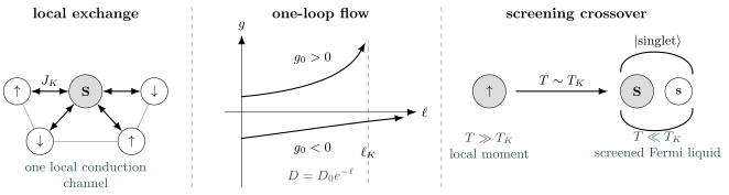
A local exchange connects the impurity to one conduction channel. Under reduction of the running cutoff, antiferromagnetic coupling grows while ferromagnetic coupling approaches zero from below. The spin-$1/2$, one-channel antiferromagnetic model crosses from a high-temperature local moment to a low-temperature screened Fermi liquid near $T_K$.

Symmetries and Conserved Quantities

For a spin-independent bath, isotropic exchange, and no magnetic field:

• conduction-electron number is conserved;
• total spin has global $SU(2)$ symmetry;
• time-reversal symmetry is present;
• charge $U(1)$ symmetry is present;
• spatial translation symmetry is broken by the impurity location.

The conserved electron number is

$$N_c = \sum_{k,\sigma} c_{k\sigma}^\dagger c_{k\sigma}.$$

The conserved total spin is

$$\mathbf J_{\mathrm{tot}} = \mathbf S + \frac12 \sum_{k,\alpha,\beta} c_{k\alpha}^\dagger \boldsymbol\sigma_{\alpha\beta} c_{k\beta},$$

so

$$\left[ H_{\mathrm K}, \mathbf J_{\mathrm{tot}} \right] =0.$$

The impurity spin alone is not conserved. Screening is a redistribution of spin correlations between impurity and bath that respects conservation of the total.

Microscopic Origin from a Local Orbital

The Kondo model is often obtained from an interacting localized orbital hybridized with a band. A representative parent Hamiltonian is

$$\begin{aligned} H_{\mathrm A} ={}& H_c + \epsilon_d \sum_\sigma n_{d\sigma} + U n_{d\uparrow}n_{d\downarrow} \\ &+ \sum_{k,\sigma} \left( V_kc_{k\sigma}^\dagger d_\sigma + \mathrm{h.c.} \right). \end{aligned}$$

In the local-moment regime,

$$\epsilon_d<0, \qquad \epsilon_d+U>0,$$

the singly occupied impurity states lie below the empty and doubly occupied states. When hybridization is weak relative to both charge-excitation energies, a Schrieffer–Wolff transformation removes virtual charge fluctuations and generates antiferromagnetic exchange.

For the normalized local-orbital convention

$$V_k = \frac{V}{\sqrt{\mathcal N}},$$

the leading exchange is

$$J_K \simeq 2\lvert V\rvert^2 \left( \frac1{\lvert\epsilon_d\rvert} + \frac1{\epsilon_d+U} \right) >0.$$

It also generates potential scattering, which vanishes at particle–hole symmetry in the simplest model. Exact numerical factors depend on the normalization of the local conduction orbital and hybridization.

This mapping explains why the Kondo Hilbert space contains a spin but no impurity charge state. It is controlled only below the eliminated charge-excitation scales. The coefficient and validity derivation belongs to Effective Hamiltonians in Many-Body Systems; the Schrieffer–Wolff Transformation owns the general method. The Anderson Impurity Model dossier owns the compact localized-level specification, charge regimes, and finite benchmark, while Anderson Impurity Model Preview owns its detailed spectral and thermodynamic structure.

Why Weak Coupling Becomes Strong

At first order, exchange scatters a conduction electron and may flip its spin together with the impurity. At higher orders, intermediate particle and hole states can lie anywhere between the observation scale $E$ and the band cutoff $D_0$.

For a smooth metallic density of states, the phase-space integral contains

$$\int_E^{D_0} \frac{d\epsilon}{\epsilon} = \ln\frac{D_0}{E}.$$

Consequently, the effective antiferromagnetic coupling has the perturbative form

$$J_{\mathrm{eff}}(E) = J_K + 2\rho_0J_K^2 \ln\frac{D_0}{E} + O(J_K^3).$$

Here $\rho_0$ is the local density of states per spin. The factor of two is convention dependent: if $\rho$ denotes the total density of states summed over both spins, the same term is written with $\rho J_K^2$.

The logarithm grows as $E$ decreases. Perturbation theory fails when

$$\rho_0J_K \ln\frac{D_0}{E} \sim1.$$

The failure does not mean that an observable physically diverges. It says that the weak-coupling expansion is being used beyond its regime.

One-Loop Scaling Flow

Let the running half-bandwidth be

$$D = D_0e^{-\ell}, \qquad \ell = \ln\frac{D_0}{D}.$$

Eliminating a thin shell of high-energy conduction states and preserving low-energy scattering gives, for the isotropic one-channel model,

$$\frac{dg}{d\ell} = 2g^2 + O(g^3),$$

where

$$g(\ell) = \rho_0J_K(\ell).$$

At one loop,

$$g(\ell) = \frac{g_0}{ 1-2g_0\ell }.$$

The flow distinguishes the two exchange signs:

Bare coupling	One-loop flow	Low-energy interpretation
$g_0>0$	grows toward strong coupling	marginally relevant antiferromagnetic exchange
$g_0<0$	approaches $0$ from below	marginally irrelevant ferromagnetic exchange
$g_0=0$	remains zero	decoupled local moment

For $g_0>0$, the one-loop denominator vanishes at a finite $\ell$. That pole marks the breakdown of weak-coupling scaling, not a literal singularity of the exact finite-temperature system.

Kondo Temperature

The one-loop breakdown scale defines the exponential structure of the Kondo energy:

$$E_K \equiv k_{\mathrm B}T_K \sim D_0 \exp \left( -\frac1{2\rho_0J_K} \right), \qquad J_K>0.$$

If $\rho_{\mathrm{tot}}=2\rho_0$ denotes the spin-summed density of states, the same exponent is

$$E_K \sim D_0 \exp \left( -\frac1{\rho_{\mathrm{tot}}J_K} \right).$$

These are the same convention, not competing physical predictions.

The exponential dependence means that a modest change in $J_K$, density of states, or cutoff can change $T_K$ by orders of magnitude. It also means that exact diagonalization with a uniformly spaced finite bath may miss screening unless its level spacing is much smaller than $E_K$.

There is no unique numerical definition

Beyond the leading weak-coupling exponent, the prefactor depends on:

• the cutoff scheme and band shape;
• whether $\rho$ is local, per spin, or spin summed;
• higher-loop conventions;
• the operational definition of $T_K$.

Common definitions use the zero-temperature impurity susceptibility, the half-width of a spectral resonance, an entropy crossover, a conductance scale, or Wilson’s numerical normalization. These definitions agree on universal scaling after a fixed conversion, but their quoted temperatures can differ by order-one factors.

Screening Crossover

For

$$k_{\mathrm B}T \gg E_K,$$

the impurity behaves approximately as a free local moment with logarithmic corrections. As the temperature or probe energy approaches $E_K$, repeated spin-flip scattering entangles the impurity with increasingly low-energy bath states.

For the ordinary spin-$1/2$, single-channel, antiferromagnetic model,

$$k_{\mathrm B}T \ll E_K$$

is a fully screened regime with no residual impurity moment. In a finite system with the compatible electron-number parity, the ground state is a global singlet. The crossover is not spontaneous symmetry breaking and has no local order parameter.

The phrase “Kondo singlet” is useful but must be interpreted carefully. At strong bare coupling, the impurity and the local conduction orbital provide an intuitive singlet benchmark. At weak bare coupling, screening involves a coherent many-electron state spread over a large range of energies and distances.

Impurity Thermodynamics

An impurity contribution is defined by subtracting the bath without the impurity:

$$X_{\mathrm{imp}} = X_{\mathrm{full}} - X_{\mathrm{bath}}.$$

This subtraction is necessary because the bath contribution is extensive while the impurity contribution is order unity.

Entropy

For a decoupled spin $S$,

$$S_{\mathrm{imp}} \longrightarrow k_{\mathrm B}\ln(2S+1)$$

at temperatures high compared with the Kondo scale but low compared with eliminated charge excitations. For the fully screened spin-$1/2$ model,

$$S_{\mathrm{imp}} \longrightarrow0$$

as $T\to0$.

The entropy is released continuously across a crossover. A finite residual impurity entropy can occur in overscreened or other nonstandard impurity fixed points, but it is not a property of the minimal one-channel spin-$1/2$ model.

Magnetic susceptibility

At high temperature, the impurity approximately obeys the Curie law

$$\chi_{\mathrm{imp}}(T) \sim \frac{ (g_{\mathrm{imp}}\mu_{\mathrm B})^2 S(S+1) }{ 3k_{\mathrm B}T }.$$

For $S=1/2$,

$$\chi_{\mathrm{imp}}(T) \sim \frac{ (g_{\mathrm{imp}}\mu_{\mathrm B})^2 }{ 4k_{\mathrm B}T }.$$

Screening cuts off the Curie divergence. At low temperature, $\chi_{\mathrm{imp}}(0)$ is finite and scales inversely with a conventionally defined $T_K$.

Heat capacity and Wilson ratio

The screened fixed point has an impurity heat capacity

$$C_{\mathrm{imp}} = \gamma_{\mathrm{imp}}T + O(T^3).$$

In the standard spin-$1/2$, single-channel Kondo normalization, the ratio of susceptibility enhancement to heat-capacity enhancement approaches the universal Wilson ratio

$$R_W = \frac{ 4\pi^2k_{\mathrm B}^2 }{ 3(g_{\mathrm{imp}}\mu_{\mathrm B})^2 } \frac{ \chi_{\mathrm{imp}}(0) }{ \gamma_{\mathrm{imp}} } =2.$$

Comparing quoted values requires checking whether the bath background, $g$-factor, and susceptibility units have been subtracted and normalized consistently.

The Screening Cloud

A spatial diagnostic is the impurity–bath spin correlation

$$C(\mathbf r) = \left\langle \mathbf S\cdot\mathbf s_c(\mathbf r) \right\rangle.$$

The crossover defines a length scale

$$\xi_K \sim \frac{ \hbar v_F }{ k_{\mathrm B}T_K },$$

where $v_F$ is an appropriate Fermi velocity. Because $T_K$ may be exponentially small, $\xi_K$ can be much larger than a microscopic lattice spacing.

The screening cloud is not one identifiable electron bound in a hydrogen-like orbital. It is a many-body correlation pattern with oscillatory, dimension-dependent, and observable-dependent structure. Finite temperature, sample size, channel geometry, and boundaries can cut it off.

In a finite spin-singlet system, the integrated bath spin compensates the impurity. For $S=1/2$, this implies the global sum rule

$$\left\langle \mathbf S\cdot \mathbf S_c^{\mathrm{tot}} \right\rangle = -\frac34,$$

provided $\mathbf S_c^{\mathrm{tot}}$ includes the full screening channel and the total state is a singlet.

Low-Energy Local Fermi Liquid

The fully screened single-channel model flows to a strong-coupling fixed point with well-defined low-energy quasiparticle scattering. The impurity is absorbed into a change of boundary condition plus irrelevant local interactions.

At particle–hole symmetry and without additional potential scattering, the zero-energy phase shift per spin is

$$\delta_\sigma(0) = \frac{\pi}{2}.$$

Potential scattering adds a nonuniversal phase shift, and asymmetric Anderson-model realizations require the corresponding Friedel-sum-rule accounting.

Low-energy corrections are analytic. A representative scattering quantity has the structure

$$\mathcal A(\omega,T) = \mathcal A(0,0) \left[ 1 - c_\omega \left( \frac{\hbar\omega}{E_K} \right)^2 - c_T \left( \frac{k_{\mathrm B}T}{E_K} \right)^2 + \cdots \right],$$

with positive coefficients whose numerical values depend on the observable and $T_K$ convention. The quadratic corrections are a hallmark of the local Fermi-liquid regime.

Observable Signatures

Dilute-alloy resistivity

At temperatures above $T_K$ but below microscopic band scales, the Kondo contribution to electron scattering grows approximately logarithmically as the system is cooled. Combined with a phonon contribution that decreases on cooling, this can produce a resistance minimum.

The perturbative logarithm cannot be extrapolated to $T=0$. In the fully screened model, scattering approaches a finite unitarity-limited value with Fermi-liquid corrections.

Spectral and scattering response

The conduction-electron $T$-matrix describes scattering from the impurity. Its low-energy resonance has a characteristic width of order $E_K$, but the Kondo model itself contains no elementary impurity-charge spectral function. A localized-electron resonance is naturally discussed in the Anderson impurity model.

Magnetic response

Static susceptibility tracks the crossover from a Curie moment to a finite screened response. Dynamic spin susceptibility probes the redistribution of spectral weight over frequencies of order $E_K/\hbar$.

Quantum-dot conductance

A quantum dot in a local-moment regime can realize Kondo correlations, and its low-temperature conductance can approach a unitary limit under symmetric coupling. The measured conductance depends on lead geometry, hybridization asymmetry, potential scattering, nonequilibrium bias, and the parent Anderson model. It is not determined by $J_K$ alone.

Controlled and Exact Limits

Zero exchange

For $J_K=0$, the bath and impurity factorize. The impurity retains entropy $k_{\mathrm B}\ln(2S+1)$ and a Curie susceptibility.

Strong antiferromagnetic exchange

When $J_K$ is much larger than the local bath hopping scale, a spin-$1/2$ impurity and one local conduction electron form a singlet with energy $-3J_K/4$. Coupling to the remaining bath can then be treated around this strong-coupling reference point.

Ferromagnetic exchange

For weak $J_K<0$, the one-loop coupling flows toward zero from below. The impurity remains asymptotically unscreened, with logarithmic corrections. This is qualitatively different from the antiferromagnetic problem.

Exactly solvable forms

The isotropic single-impurity model admits Bethe-ansatz solutions after reducing the coupled conduction channel to an effective one-dimensional radial problem. These solutions provide exact thermodynamics and confirm the crossover between weak and strong coupling.

Exact solvability depends on model structure. Adding arbitrary band shapes, several impurities, channel asymmetry, or general nonequilibrium driving need not preserve integrability.

Numerical and Analytical Methods

Perturbative renormalization

Poor-man’s scaling and field-theoretic RG organize the high-energy regime where the running coupling remains small. They determine the exponential scale and universal logarithms but do not justify using a truncated weak-coupling series deep below $T_K$.

Numerical renormalization group

Wilson’s numerical renormalization group logarithmically discretizes the bath and maps it to a chain with decreasing energy scales. A representative asymptotic hopping is

$$t_n \propto D_0 \Lambda^{-n/2}, \qquad \Lambda>1.$$

Iterative diagonalization then resolves exponentially separated impurity scales. Discretization, state truncation, broadening, and $z$-averaging must be converged for quantitative spectra.

Bethe ansatz

Bethe ansatz gives exact equilibrium results for integrable versions. It is especially powerful for thermodynamics and universal ratios, but extracting arbitrary real-frequency observables or nonintegrable perturbations can remain difficult.

Tensor networks and finite baths

Matrix-product-state and related methods can resolve real-space screening correlations after mapping the bath to a chain. Finite-size level spacing, chain length, bath discretization, and entanglement growth must all be compared with $E_K$ and $\xi_K$.

Quantum Monte Carlo

Impurity Monte Carlo methods can be highly effective for Anderson-type formulations. Analytic continuation from imaginary time is ill-conditioned, and sign or ergodicity difficulties depend on the chosen variant.

Principal Variants

Anisotropic exchange

The axial model is

$$H_{\mathrm{int}} = J_\perp \left( S^xs_0^x + S^ys_0^y \right) + J_zS^zs_0^z.$$

Its coupled scaling equations reveal flows toward isotropy in part of the antiferromagnetic regime and connect to boundary sine-Gordon and spin-boson descriptions. The general fixed-point and phase-portrait language belongs in Renormalization Group Preview.

Higher impurity spin and several channels

For $K$ equivalent screening channels and impurity spin $S$:

• $K=2S$ suggests exact screening;
• $K<2S$ gives underscreening and a residual moment;
• $K>2S$ gives overscreening and can produce a non-Fermi-liquid fixed point.

These rules assume channel symmetry and antiferromagnetic coupling. Channel anisotropy, potential scattering, and additional interactions can destabilize special fixed points.

Two impurities and Kondo lattices

Two or more moments can interact indirectly through the conduction bath. The induced RKKY scale is schematically

$$E_{\mathrm{RKKY}} \sim J_K^2 \chi_c(R),$$

where $\chi_c(R)$ is the spatial conduction spin susceptibility.

Competition between intermoment correlations and Kondo screening is absent from the one-impurity model. In a Kondo lattice, coherence, magnetism, heavy quasiparticles, and possible Kondo-breakdown phenomena require a distinct many-body analysis.

RKKY Interaction owns the sign and normalization ledger, Lindhard range function, Fermi-surface geometry, and ordering consequences of this induced exchange.

Nonmetallic baths

If the local density of states vanishes or diverges at the Fermi energy, the constant-$\rho_0$ logarithmic analysis changes. Pseudogap, superconducting, Luttinger-liquid, and topological baths can support impurity quantum phase transitions or altered screening.

The metallic formula for $T_K$ must not be transplanted unchanged into these cases.

Model Boundaries

The minimal Kondo Hamiltonian omits:

• impurity empty and doubly occupied charge states;
• explicit orbital hybridization;
• impurity motion;
• electron–electron interactions in the bath;
• phonons, disorder, and nonequilibrium reservoirs;
• interimpurity exchange and lattice coherence;
• channel anisotropy unless added;
• finite-range or momentum-dependent exchange unless added.

If an observable directly probes impurity charge fluctuations or Hubbard satellites, the Kondo Hilbert space is too small. If many moments interact coherently, a single-impurity solution is not a Kondo-lattice solution.

Common Mistakes

Treating the bath as one electron

The local singlet benchmark fixes the exchange sign, but the weak-coupling Kondo state is a many-electron entangled state.

Omitting the cutoff and density-of-states convention

A quoted $J_K$ does not determine $T_K$ without a band, local density of states, and normalization.

Mixing per-spin and total densities of states

This changes the factor of two in the exponent if the coupling definition is left unchanged. State which $\rho$ is used.

Calling the one-loop pole a physical divergence

The pole marks breakdown of weak-coupling perturbation theory and crossover toward a finite strong-coupling fixed point.

Assuming every exchange is screened

Weak ferromagnetic coupling is marginally irrelevant. Screening also depends on impurity spin, channel count, and bath density of states.

Equating screening with magnetic order

Single-impurity Kondo screening is a crossover to an entangled singlet, not spontaneous symmetry breaking.

Using a unique universal Kondo temperature

Different operational definitions differ by fixed factors. Universal curves can be compared only after the convention is aligned.

Confusing the Kondo model with its Anderson parent

The Kondo model has no impurity charge dynamics. Hybridization resonances and charge excitations belong to the Anderson formulation.

Applying the single-impurity result to a lattice

RKKY interactions, coherence, and collective phases introduce scales absent from the one-impurity model.

Extrapolating logarithmic resistivity to zero temperature

Perturbative logarithms are valid above the strong-coupling crossover. The screened low-temperature regime is a local Fermi liquid.

Worked Example: One-Loop Scale

Suppose the per-spin dimensionless coupling is

$$g_0 = \rho_0J_K = 0.08.$$

The one-loop scale is

$$\frac{E_K}{D_0} \sim \exp \left( -\frac1{2g_0} \right) = e^{-6.25} \approx 1.93\times10^{-3}.$$

A bare coupling of order $10^{-1}$ therefore produces a scale of order $10^{-3}D_0$. This separation explains both the power of logarithmic methods and the numerical difficulty of resolving $T_K$ with a uniformly spaced bath.

Worked Example: Particle–Hole-Symmetric Parent

For

$$\epsilon_d = -\frac U2,$$

the two virtual charge-excitation costs are equal:

$$\lvert\epsilon_d\rvert = \epsilon_d+U = \frac U2.$$

The simple Schrieffer–Wolff result becomes

$$J_K \simeq \frac{8\lvert V\rvert^2}{U}.$$

The potential-scattering contributions from empty and doubly occupied virtual states cancel in the particle–hole-symmetric convention. The exchange contributions add, so the low-energy coupling is antiferromagnetic.

Exercises

Exercise 1: Singlet–triplet splitting

For an impurity spin $1/2$ and one singly occupied local conduction orbital, derive the exchange energies and identify the favored state for each sign of $J_K$.

Solution

Use

$$\mathbf S\cdot\mathbf s_0 = \frac12 \left( \mathbf J^2 -\mathbf S^2 -\mathbf s_0^2 \right).$$

For the singlet, $J=0$, while $S=s_0=1/2$. Therefore

$$\mathbf S\cdot\mathbf s_0 = -\frac34.$$

For the triplet, $J=1$, giving

$$\mathbf S\cdot\mathbf s_0 = +\frac14.$$

Hence

$$E_{\mathrm s} = -\frac34J_K, \qquad E_{\mathrm t} = +\frac14J_K.$$

The singlet is favored for $J_K>0$ and the triplet for $J_K<0$.

Exercise 2: Solve the one-loop flow

Integrate $dg/d\ell=2g^2$ with $g(0)=g_0$. Describe the flows for positive and negative $g_0$.

Solution

Separate variables:

$$\frac{dg}{g^2} = 2\,d\ell.$$

Integrating gives

$$-\frac1{g(\ell)} + \frac1{g_0} = 2\ell,$$

so

$$g(\ell) = \frac{g_0}{ 1-2g_0\ell }.$$

For $g_0>0$, the running coupling grows and the one-loop expression breaks down at $\ell=1/(2g_0)$. For $g_0<0$, the denominator grows without vanishing and $g(\ell)\to0^-$.

Exercise 3: Convert density-of-states conventions

Show that

$$D_0e^{-1/(2\rho_0J_K)}$$

with $\rho_0$ per spin equals

$$D_0e^{-1/(\rho_{\mathrm{tot}}J_K)}$$

when $\rho_{\mathrm{tot}}=2\rho_0$.

Solution

Substitute

$$\rho_{\mathrm{tot}} = 2\rho_0.$$

Then

$$\frac1{\rho_{\mathrm{tot}}J_K} = \frac1{2\rho_0J_K}.$$

The exponents are identical. A factor-of-two disagreement appears only when the symbol $\rho$ is redefined without changing the displayed formula.

Exercise 4: Impurity Curie law

Evaluate the high-temperature Curie susceptibility for a spin-$1/2$ impurity with magnetic moment $g_{\mathrm{imp}}\mu_{\mathrm B}\mathbf S$.

Solution

For a free spin in a weak field along $z$,

$$\chi = \frac{ (g_{\mathrm{imp}}\mu_{\mathrm B})^2 }{ k_{\mathrm B}T } \left\langle (S^z)^2 \right\rangle.$$

An unpolarized spin-$1/2$ has

$$\left\langle (S^z)^2 \right\rangle = \frac14.$$

Therefore

$$\chi_{\mathrm{imp}} = \frac{ (g_{\mathrm{imp}}\mu_{\mathrm B})^2 }{ 4k_{\mathrm B}T }.$$

Kondo correlations add logarithmic corrections at high temperature and cut off the divergence below the screening scale.

Exercise 5: Antiferromagnetic exchange from a local orbital

In the local-moment regime $\epsilon_d<0<\epsilon_d+U$, explain why the leading Schrieffer–Wolff exchange is positive.

Solution

The virtual empty-state cost is $\lvert\epsilon_d\rvert>0$, and the virtual doublon cost is $\epsilon_d+U>0$. In the stated convention,

$$J_K \simeq 2\lvert V\rvert^2 \left( \frac1{\lvert\epsilon_d\rvert} + \frac1{\epsilon_d+U} \right).$$

Both denominators and the prefactor are positive, so $J_K>0$. Empty and doubly occupied virtual processes both contribute to antiferromagnetic spin exchange even though their potential-scattering contributions can have opposite signs.

Exercise 6: Screening length estimate

Take $v_F=1.0\times10^6\,\mathrm{m\,s^{-1}}$ and $T_K=10\,\mathrm K$. Estimate $\xi_K=\hbar v_F/(k_{\mathrm B}T_K)$.

Solution

Using

$$\hbar \approx 1.055\times10^{-34}\,\mathrm{J\,s}$$

and

$$k_{\mathrm B} \approx 1.381\times10^{-23}\,\mathrm{J\,K^{-1}},$$

one obtains

$$\xi_K \approx \frac{ 1.055\times10^{-34} \times 1.0\times10^6 }{ 1.381\times10^{-23} \times 10 } \mathrm m.$$

Thus

$$\xi_K \approx 7.6\times10^{-7}\,\mathrm m = 0.76\,\mu\mathrm m.$$

The result is much larger than an atomic spacing, illustrating why direct spatial observation of the screening cloud is subtle.

Exercise 7: Identify the missing physics

For each claim, state whether the minimal single-impurity Kondo model is sufficient:

1. the high-temperature Curie response of one local moment;
2. the energy of an impurity doublon;
3. competition between Kondo screening and magnetic order in a lattice;
4. the sign of the isolated exchange singlet–triplet splitting.

Solution

1. Yes, within the temperature window below eliminated charge scales.
2. No. The impurity doublon is absent; an Anderson-type model is required.
3. No. Intermoment interactions and lattice coherence are absent.
4. Yes. The local exchange benchmark determines the sign convention directly.

Summary

• The Kondo model couples a localized spin to a local conduction-electron spin density.
• With $H_{\mathrm{int}}=J_K\mathbf S\cdot\mathbf s_0$, positive $J_K$ is antiferromagnetic.
• Spin-flip exchange generates logarithmic corrections that make weak antiferromagnetic coupling grow at low energy.
• With a per-spin local density of states, one-loop scaling gives $E_K\sim D_0e^{-1/(2\rho_0J_K)}$.
• Numerical values of $T_K$ depend on cutoff, density-of-states, and operational conventions.
• A spin-$1/2$ impurity in one metallic channel crosses from a local moment to a screened local Fermi liquid.
• The screening cloud is a many-electron correlation pattern with scale $\xi_K\sim\hbar v_F/(k_{\mathrm B}T_K)$.
• Ferromagnetic exchange, several channels, higher spin, nonmetallic baths, and Kondo lattices can have qualitatively different infrared behavior.

Further Reading

• Kondo Effect
• RKKY Interaction
• Kondo Model
• Anderson Impurity Model
• Common Many-Body Hamiltonians
• Anderson Impurity Model Preview
• Fermionic Operators in Many-Body Models
• Density and Current Operators
• Effective Hamiltonians in Many-Body Systems
• Schrieffer–Wolff Transformation
• Correlation Functions Overview
• Fluctuations and Susceptibilities
• Why Many-Body QM Leads to QFT
• Condensed Matter Roadmap

References

1. J. Kondo, “Resistance Minimum in Dilute Magnetic Alloys,” Progress of Theoretical Physics 32, 37–49 (1964), doi:10.1143/PTP.32.37.
2. J. R. Schrieffer and P. A. Wolff, “Relation between the Anderson and Kondo Hamiltonians,” Physical Review 149, 491–492 (1966), doi:10.1103/PhysRev.149.491.
3. P. W. Anderson, “A Poor Man’s Derivation of Scaling Laws for the Kondo Problem,” Journal of Physics C: Solid State Physics 3, 2436–2441 (1970), doi:10.1088/0022-3719/3/12/008.
4. K. G. Wilson, “The Renormalization Group: Critical Phenomena and the Kondo Problem,” Reviews of Modern Physics 47, 773–840 (1975), doi:10.1103/RevModPhys.47.773.
5. P. Nozières, “A Fermi-Liquid Description of the Kondo Problem at Low Temperatures,” Journal of Low Temperature Physics 17, 31–42 (1974), doi:10.1007/BF00654541.
6. N. Andrei, “Diagonalization of the Kondo Hamiltonian,” Physical Review Letters 45, 379–382 (1980), doi:10.1103/PhysRevLett.45.379.
7. N. Andrei, K. Furuya, and J. H. Lowenstein, “Solution of the Kondo Problem,” Reviews of Modern Physics 55, 331–402 (1983), doi:10.1103/RevModPhys.55.331.
8. I. Affleck and P. Simon, “Detecting the Kondo Screening Cloud Around a Quantum Dot,” Physical Review Letters 86, 2854–2857 (2001), doi:10.1103/PhysRevLett.86.2854.
9. R. Bulla, T. A. Costi, and T. Pruschke, “Numerical Renormalization Group Method for Quantum Impurity Systems,” Reviews of Modern Physics 80, 395–450 (2008), doi:10.1103/RevModPhys.80.395.
10. A. C. Hewson, The Kondo Problem to Heavy Fermions, Cambridge University Press (1993).