Anderson Impurity Model Preview

The single-impurity Anderson model describes a spinful localized orbital that can be empty, singly occupied, or doubly occupied while exchanging particles with a fermionic bath. Its minimal equilibrium Hamiltonian is

$$\begin{aligned} H_{\mathrm A} &= \sum_{k,\sigma} \epsilon_k c_{k\sigma}^{\dagger}c_{k\sigma} + \epsilon_d \sum_\sigma n_{d\sigma} + U n_{d\uparrow}n_{d\downarrow} \\ &\quad+ \sum_{k,\sigma} \left( V_k c_{k\sigma}^{\dagger}d_\sigma + V_k^* d_\sigma^{\dagger}c_{k\sigma} \right), \end{aligned}$$

where $n_{d\sigma}=d_\sigma^\dagger d_\sigma$. Throughout this page, $\epsilon_k$ and $\epsilon_d$ are measured relative to the equilibrium chemical potential. Equivalently, the displayed operator is the grand-canonical generator $H_{\mathrm{physical}}-\mu N$ up to an irrelevant constant.

Three ingredients do distinct jobs:

• $\epsilon_d$ sets the energy of the localized orbital;
• $U$ penalizes simultaneous occupation by both spins;
• $V_k$ allows coherent charge transfer between the orbital and bath.

The model is a meeting point for localized charge, local moments, resonant scattering, the Kondo effect, quantum-dot transport, and dynamical mean-field theory. It is also a useful lesson in model discipline: the bath cannot be summarized by a density of states alone, and the impurity cannot always be replaced by a spin.

Canonical Scope

This page is the canonical teaching treatment. It owns:

• the single-orbital Anderson Hamiltonian and its conventions;
• the four impurity charge states and atomic charge regimes;
• the bath hybridization function;
• the exactly solvable noninteracting resonant level;
• the interacting impurity Green function and qualitative spectral structure;
• criteria for the local-moment and mixed-valence regimes;
• the controlled handoff to the Kondo model;
• impurity observables, solution methods, and a DMFT preview.

The Anderson Impurity Model dossier owns the compact reproducible specification, regime and exact-status map, observable–method dictionary, and exact two-orbital finite-bath benchmark. This page develops the associated physics and derivations. Kondo Effect carries the resulting local-moment regime into dilute-alloy transport, quantum-dot diagnostics, screening experiments, and heavy-fermion materials.

It does not rederive the general unitary block diagonalization that eliminates impurity charge states. That method belongs to the Schrieffer–Wolff Transformation. The comparative charge-path derivation, including exchange and potential scattering, is in Effective Hamiltonians in Many-Body Systems. The resulting spin-only model specification, controlled limits, and finite benchmark belong to the Kondo Model dossier. Its logarithmic flow, screening cloud, and low-energy local Fermi liquid belong to the Kondo Model Preview.

The page also does not develop the general many-body Green-function formalism. Green Functions in Many-Body QM owns addition and removal sectors, Lehmann weights, spectral sum rules, and the Matsubara bridge. Retarded and Advanced Green Functions and Spectral Representation of Green Functions supply the underlying boundary-value and resolvent background; the formulas below specialize those conventions to one localized orbital.

Polarons Preview owns the contrasting mobile-impurity problem, where recoil and a conserved total momentum organize a particle plus its environmental cloud. The Anderson orbital is fixed in space and exchanges particles with its bath instead.

Why Retain Impurity Charge?

A Kondo Hamiltonian starts with a localized spin and therefore assumes that the impurity charge has already been frozen. The Anderson model asks an earlier question: when does a localized orbital form a moment at all?

That question requires the empty, singly occupied, and doubly occupied sectors. Virtual transitions among them generate exchange at low energy, while real charge fluctuations produce mixed valence, Coulomb-blockade features, and resonant-level physics. The Anderson model can therefore describe both the emergence of a local moment and its eventual screening by a metal.

The word impurity means that one distinguished local degree of freedom is embedded in a much larger host. It need not represent literal chemical contamination. The same Hamiltonian can model:

• a magnetic atom in a metal;
• a gate-tunable quantum-dot level coupled to leads;
• a molecular orbital near electrodes;
• an adsorbate coupled to a surface band;
• the auxiliary correlated site in a DMFT calculation.

Which interpretation is intended determines how $\epsilon_d$, $U$, the bath, and measured observables map to laboratory quantities.

Degrees of Freedom and Hilbert Space

The bath has fermion modes $c_{k\sigma}$ and the localized orbital has modes $d_\sigma$, with

$$\{d_\sigma,d_{\sigma'}^\dagger\} = \delta_{\sigma\sigma'}, \qquad \{c_{k\sigma},c_{k'\sigma'}^\dagger\} = \delta_{kk'}\delta_{\sigma\sigma'},$$

and all impurity operators anticommute with all bath operators. After a global ordering of the modes is chosen, the many-body basis is the occupation-number basis described in Fermionic Operators in Many-Body Models.

The impurity sector alone has four states:

$$\lvert0\rangle, \qquad \lvert\uparrow\rangle = d_\uparrow^\dagger\lvert0\rangle, \qquad \lvert\downarrow\rangle = d_\downarrow^\dagger\lvert0\rangle,$$ $$\lvert2\rangle = d_\uparrow^\dagger d_\downarrow^\dagger \lvert0\rangle.$$

The phase of $\lvert2\rangle$ depends on the chosen mode order, but all physical predictions are independent of that convention.

The impurity charge and spin are

$$n_d = n_{d\uparrow}+n_{d\downarrow},$$ $$\mathbf S_d = \frac12 \sum_{\alpha,\beta} d_\alpha^\dagger \boldsymbol\sigma_{\alpha\beta} d_\beta.$$

An identity useful for diagnosing moment formation is

$$\mathbf S_d^2 = \frac34 \left( n_d-2n_{d\uparrow}n_{d\downarrow} \right).$$

It vanishes in the empty and doubly occupied states and equals $3/4$ in either singly occupied state.

The Atomic Limit

Set every $V_k$ to zero. The four impurity energies are then

$$E_0=0, \qquad E_\uparrow=E_\downarrow=\epsilon_d, \qquad E_2=2\epsilon_d+U.$$

For repulsive $U>0$, the zero-temperature ground-state charge changes at two degeneracy points:

$$\begin{array}{c|c} \text{parameter range} & \text{atomic ground-state charge} \\ \hline \epsilon_d>0 & n_d=0 \\ -U<\epsilon_d<0 & n_d=1 \\ \epsilon_d<-U & n_d=2 \end{array}$$

Inside the singly occupied interval, the energy costs for virtual charge fluctuations are

$$E_0-E_\sigma = -\epsilon_d, \qquad E_2-E_\sigma = \epsilon_d+U.$$

Both are positive when

$$\epsilon_d<0<\epsilon_d+U.$$

This is the atomic local-moment window. Hybridization rounds the sharp charge steps into crossovers, but the two charge-excitation energies remain the natural scales for deciding whether a spin-only reduction is controlled.

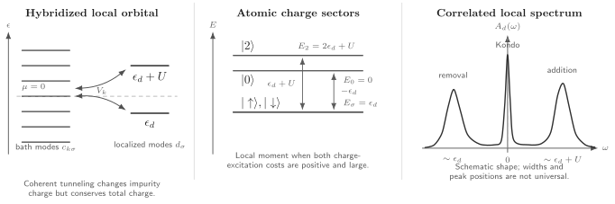
The single-impurity Anderson model in three complementary views. Left: a localized orbital exchanges fermions coherently with a bath. Center: the atomic energies expose the empty, spin-doublet, and doubly occupied sectors and their charge gaps. Right: in a correlated metallic local-moment regime, the impurity spectrum can show broad charge-transfer features together with a much narrower low-energy Kondo resonance. The spectral panel is schematic rather than a universal line shape.

Thermal Atomic Benchmark

The isolated impurity partition function is

$$Z_d = 1 + 2e^{-\beta\epsilon_d} + e^{-\beta(2\epsilon_d+U)}.$$

It gives

$$\langle n_d\rangle = \frac{ 2e^{-\beta\epsilon_d} + 2e^{-\beta(2\epsilon_d+U)} }{Z_d},$$ $$\langle n_{d\uparrow}n_{d\downarrow}\rangle = \frac{e^{-\beta(2\epsilon_d+U)}}{Z_d}.$$

The probability of single occupation is

$$P_1 = \frac{2e^{-\beta\epsilon_d}}{Z_d} = \left\langle n_d-2n_{d\uparrow}n_{d\downarrow} \right\rangle.$$

These formulas are exact only at $V_k=0$. They are nevertheless valuable checks for numerical impurity solvers and for understanding entropy plateaus when hybridization is weak.

Bath Data Beyond a Density of States

The free bath Hamiltonian is diagonal in the chosen $k$ basis,

$$H_{\mathrm{bath}} = \sum_{k,\sigma} \epsilon_k c_{k\sigma}^\dagger c_{k\sigma}.$$

The impurity does not couple equally to every bath wave function. It couples through the amplitudes $V_k$. For a finite discretization, define

$$V_{\mathrm{loc}}^2 = \sum_k\lvert V_k\rvert^2,$$

and, when $V_{\mathrm{loc}}\ne0$,

$$f_{0\sigma} = \frac1{V_{\mathrm{loc}}} \sum_k V_k c_{k\sigma}.$$

Then

$$H_{\mathrm{hyb}} = V_{\mathrm{loc}} \sum_\sigma \left( f_{0\sigma}^\dagger d_\sigma + d_\sigma^\dagger f_{0\sigma} \right).$$

Only this local combination couples directly to the impurity. Orthogonal bath combinations still matter because the bath Hamiltonian propagates amplitude away from and back to $f_{0\sigma}$. This observation underlies the chain representation used by numerical renormalization group and tensor-network methods.

In a continuum normalization, $V_{\mathrm{loc}}^2$ by itself may be cutoff dependent. The invariant object for impurity dynamics is the hybridization function.

Hybridization Function

For complex frequency $z$ off the bath spectrum, define

$$\Delta(z) = \sum_k \frac{\lvert V_k\rvert^2}{z-\epsilon_k}.$$

Its retarded boundary value is written

$$\Delta^R(\omega) = \Lambda(\omega)-i\Gamma(\omega),$$

where

$$\Gamma(\omega) = \pi \sum_k \lvert V_k\rvert^2 \delta(\omega-\epsilon_k) \ge0,$$

and

$$\Lambda(\omega) = \operatorname{P} \sum_k \frac{\lvert V_k\rvert^2}{\omega-\epsilon_k}.$$

The imaginary part $\Gamma$ measures broadening into available bath states. The real part $\Lambda$ shifts the orbital energy. Causality ties them by a Hilbert transform, so choosing one frequency dependence fixes the other up to subtraction conventions.

If

$$V_k = \frac{V}{\sqrt{\mathcal N}}$$

and the per-spin bath density of states is

$$\rho_0(\omega) = \frac1{\mathcal N} \sum_k\delta(\omega-\epsilon_k),$$

then

$$\Gamma(\omega) = \pi\lvert V\rvert^2\rho_0(\omega).$$

This formula fixes a common factor-of-two ambiguity: $\rho_0$ is per spin. Summing the bath density over both spin species would double it, while $\Gamma$ for one spin channel would remain unchanged.

Wide-band convention

A common idealization takes a broad, particle–hole-symmetric band with nearly constant

$$\Gamma(\omega) \simeq \Gamma$$

over all frequencies relevant to the impurity. A constant part of $\Lambda$ can then be absorbed into a redefined $\epsilon_d$.

In this convention, $\Gamma$ is the half-width at half maximum of the noninteracting impurity spectral peak. Some transport literature defines a linewidth equal to $2\Gamma$ or assigns $\Gamma_L+\Gamma_R$ differently. A numerical value is meaningless until the definition is stated.

Conserved Quantities and Symmetries

Hybridization does not conserve the impurity charge or bath charge separately:

$$[H_{\mathrm A},n_d] \ne0, \qquad [H_{\mathrm A},N_{\mathrm{bath}}] \ne0.$$

It does conserve their sum,

$$N = n_d + \sum_{k,\sigma} c_{k\sigma}^\dagger c_{k\sigma}, \qquad [H_{\mathrm A},N]=0.$$

With spin-independent $\epsilon_k$, $V_k$, $\epsilon_d$, and $U$, the model has global spin $SU(2)$ symmetry. It also has time-reversal symmetry in the absence of magnetic fields and complex fluxes that cannot be gauged away. The impurity breaks spatial translation symmetry even when the host is translationally invariant.

The phases of the $V_k$ are often removable by redefining bath modes, but not every phase is unphysical in multilead or interferometric geometries. Gauge choices should be separated from measurable loop phases.

Particle–Hole Symmetry

Suppose the bath and hybridization spectrum are particle–hole symmetric about zero energy. The impurity is particle–hole symmetric when

$$\epsilon_d = -\frac U2.$$

The atomic energies then obey

$$E_0=E_2=0, \qquad E_\uparrow=E_\downarrow=-\frac U2.$$

The full symmetric model has

$$\langle n_d\rangle=1$$

at equilibrium and zero field. This is an expectation value, not a statement that the impurity is always singly occupied. For finite hybridization,

$$P_0=P_2$$

while both probabilities can be nonzero. Charge fluctuations survive even though their average is balanced.

Particle–hole symmetry also removes the leading potential-scattering term generated in the Kondo reduction. Away from symmetry, that term is generally present.

Exactly Solvable Resonant Level

Set $U=0$. The Hamiltonian is quadratic, and the retarded impurity Green function is exactly

$$G_{d\sigma}^R(\omega) = \frac1{ \omega-\epsilon_d-\Lambda(\omega) +i\Gamma(\omega) }.$$

Using the convention

$$A_{d\sigma}(\omega) = -\frac1\pi \operatorname{Im}G_{d\sigma}^R(\omega),$$

the spectral function is

$$A_{d\sigma}(\omega) = \frac1\pi \frac{\Gamma(\omega)}{ [\omega-\epsilon_d-\Lambda(\omega)]^2 +\Gamma(\omega)^2 }.$$

For a wide symmetric band with $\Lambda=0$ and constant $\Gamma$,

$$A_{d\sigma}(\omega) = \frac1\pi \frac{\Gamma}{ (\omega-\epsilon_d)^2+\Gamma^2 }.$$

This is a Lorentzian centered at $\epsilon_d$ with full width $2\Gamma$. Hybridization has converted the discrete local level into a resonance while preserving the single-orbital sum rule

Spectral Functions owns the general HWHM/FWHM, lifetime, residue, and resolution-convolution dictionary; this section owns the resonant-level benchmark.

$$\int_{-\infty}^{\infty} d\omega\, A_{d\sigma}(\omega) =1.$$

The equilibrium occupation is

$$\langle n_{d\sigma}\rangle = \int_{-\infty}^{\infty} d\omega\, f(\omega)A_{d\sigma}(\omega).$$

At zero temperature in the ideal wide-band limit,

$$\langle n_{d\sigma}\rangle = \frac12 - \frac1\pi \arctan\frac{\epsilon_d}{\Gamma}.$$

Thus charge changes continuously over a scale of order $\Gamma$. This solvable limit provides the baseline from which interaction effects should be identified.

Interacting Impurity Green Function

For $U\ne0$, write the exact Dyson form

$$G_{d\sigma}(z) = \frac1{ z-\epsilon_d-\Delta(z)-\Sigma_\sigma(z) }.$$

Here $\Delta$ contains all effects of the noninteracting bath, while $\Sigma_\sigma$ is the proper self-energy generated by $U$. This separation is essential:

• $\Delta$ is input data defining the environment;
• $\Sigma$ is an interacting output of the impurity problem.

The large-frequency behavior

$$G_{d\sigma}(z) = \frac1z + O\!\left(\frac1{z^2}\right)$$

enforces the unit spectral sum rule. More detailed high-frequency moments encode $\epsilon_d$, $U$, occupancy, and hybridization and are valuable numerical checks.

The interaction self-energy is generally frequency dependent. Replacing it by only a static Hartree shift,

$$\Sigma_\sigma^{\mathrm H} = U\langle n_{d\bar\sigma}\rangle,$$

cannot reproduce the full separation of charge and spin scales. An unrestricted static mean field may also display a spin-polarized impurity solution even though the exact finite single-impurity equilibrium state preserves spin symmetry at zero field.

Atomic Green Function as a Check

At $V_k=0$, the opposite-spin occupation commutes with the impurity Hamiltonian. The exact atomic Green function is

$$G_{d\sigma}^{\mathrm{at}}(z) = \frac{1-\langle n_{d\bar\sigma}\rangle}{z-\epsilon_d} + \frac{\langle n_{d\bar\sigma}\rangle}{z-\epsilon_d-U}.$$

It has two addition or removal energies, not a single Hartree-shifted pole. In the paramagnetic particle–hole-symmetric atomic local-moment state, the two poles have equal weight and lie at

$$\omega=-\frac U2, \qquad \omega=+\frac U2.$$

Finite hybridization broadens and shifts these atomic features and, at sufficiently low temperature in a metallic bath, creates additional low-energy many-body structure.

Spectral Anatomy in the Correlated Regime

In a broad metallic bath with

$$U\gg\Gamma, \qquad \epsilon_d<0<\epsilon_d+U,$$

the low-temperature impurity spectrum often has three recognizable energy regions:

1. a lower charge-transfer feature associated roughly with removing the impurity electron;
2. an upper charge-transfer feature associated roughly with adding a second electron;
3. a narrow low-energy Kondo resonance associated with coherent spin screening.

The broad features are often called lower and upper Hubbard satellites. Their centers are near $\epsilon_d$ and $\epsilon_d+U$ only in an approximate sense; real-part shifts, asymmetry, and strong mixing can move and distort them.

The low-energy resonance is not an extra one-particle state placed on top of the original orbital. Spectral weight is redistributed while

$$\int d\omega\,A_{d\sigma}(\omega)=1$$

remains fixed. Its width is controlled by a low-energy many-body scale, whereas the satellites reflect charge-excitation scales. This separation is one of the clearest signatures of correlated impurity physics.

The familiar three-feature picture is not universal. It can disappear or change qualitatively for weak $U$, mixed valence, strongly energy-dependent baths, pseudogaps, superconducting gaps, several orbitals, or temperatures above the screening scale.

Charge Regimes with Finite Hybridization

At nonzero $V_k$, impurity charge is not a good quantum number. The atomic sectors become crossover regimes.

Empty-orbital regime

If $\epsilon_d$ lies well above the Fermi energy compared with $\Gamma$ and temperature, then

$$\langle n_d\rangle\ll1.$$

The impurity behaves primarily as an unoccupied resonance.

Local-moment regime

If

$$-\epsilon_d \gg \Gamma,k_{\mathrm B}T,$$

and

$$\epsilon_d+U \gg \Gamma,k_{\mathrm B}T,$$

then empty and double states are costly, $\langle n_d\rangle$ is near one, and the impurity supports a well-formed spin over an intermediate energy window.

Mixed-valence regime

If either charge-excitation energy is comparable to $\Gamma$, real and virtual charge fluctuations are strong. The occupancy is noninteger and no clean scale separation justifies discarding the empty or doubly occupied sector.

Doubly occupied regime

If $\epsilon_d+U$ lies well below the Fermi energy, then

$$\langle n_d\rangle\simeq2.$$

The localized orbital is nearly full and carries little spin.

These are crossovers for the ordinary single-orbital model with a featureless metallic bath, not distinct thermodynamic phases.

From Anderson to Kondo

Deep in the local-moment regime, hybridization changes the impurity charge only virtually. A Schrieffer–Wolff transformation projects onto the singly occupied impurity doublet.

For

$$V_k = \frac{V}{\sqrt{\mathcal N}},$$

and the Kondo convention

$$H_{\mathrm{int}} = J_K\mathbf S_d\cdot\mathbf s_0,$$

the leading exchange at the Fermi surface is

$$J_K \simeq 2\lvert V\rvert^2 \left( \frac1{-\epsilon_d} + \frac1{\epsilon_d+U} \right) >0.$$

Both virtual paths generate antiferromagnetic exchange: one visits the empty state and the other visits the doubly occupied state. The transformation also generates potential scattering away from particle–hole symmetry.

At the symmetric point,

$$\epsilon_d=-\frac U2,$$

so

$$J_K \simeq \frac{8\lvert V\rvert^2}{U}.$$

This mapping is controlled only at energies well below

$$E_{\mathrm{charge}} = \min\left(-\epsilon_d,\epsilon_d+U\right)$$

and when hybridization is small compared with both denominators. It is not controlled in mixed valence or at a charge degeneracy.

The projection changes the Hilbert space. The Anderson model retains impurity charge, charge-transfer peaks, and gate-dependent valence; the Kondo model retains only the local spin and its exchange with conduction electrons.

Kondo Scale in Anderson Parameters

For a wide flat metallic band in the local-moment regime, a commonly used asymptotic estimate is

$$k_{\mathrm B}T_K \sim \sqrt{\frac{U\Gamma}{2}} \exp\!\left[ \frac{\pi\epsilon_d(\epsilon_d+U)} {2U\Gamma} \right].$$

At particle–hole symmetry this becomes

$$k_{\mathrm B}T_K \sim \sqrt{\frac{U\Gamma}{2}} \exp\!\left( -\frac{\pi U}{8\Gamma} \right).$$

These expressions display the crucial exponential separation between charge and spin scales. They are not universal equalities. Prefactors change with the definition of $T_K$, bandwidth, cutoff scheme, and hybridization convention. Near mixed valence, the asymptotic local-moment formula should not be used.

The Kondo Model Preview owns the scaling flow and the operational meanings of the Kondo temperature.

Static Observables

Several local observables distinguish the impurity regimes.

Occupancy

$$n_d = \sum_\sigma \langle n_{d\sigma}\rangle.$$

It tracks valence but does not by itself distinguish coherent screening from an unscreened local moment.

Double occupancy

$$D_d = \langle n_{d\uparrow}n_{d\downarrow}\rangle.$$

Repulsive $U$ suppresses $D_d$, but hybridization keeps it finite except in a strict projected or infinite-$U$ limit.

Instantaneous local moment

$$m_{\mathrm{loc}}^2 = \left\langle (n_{d\uparrow}-n_{d\downarrow})^2 \right\rangle = n_d-2D_d.$$

This measures the probability of single occupation. It can remain large even when the long-time moment is Kondo screened. An instantaneous moment and a free Curie moment are not the same diagnostic.

Charge and spin susceptibilities

With sources coupled to $n_d$ and $S_d^z$, static susceptibilities probe the response of valence and magnetization. In the local-moment crossover, charge response is suppressed before spin response becomes screened. The general fluctuation and response conventions belong to Fluctuations and Susceptibilities.

Impurity Thermodynamics

Impurity thermodynamic quantities are normally defined by subtracting the free bath contribution from the full coupled system. This subtraction matters because hybridization rearranges bath states as well as impurity states.

For a well-separated local-moment regime, cooling can reveal the sequence

$$\ln4 \longrightarrow \ln2 \longrightarrow 0$$

in the impurity entropy:

• $\ln4$ when all four impurity charge states are thermally accessible;
• $\ln2$ when charge is frozen but the spin doublet remains effectively free;
• $0$ when a single-channel metallic bath screens the spin into a nondegenerate Fermi-liquid ground state.

The plateaus require separated scales and need not be sharp. In a finite bath, pseudogapped bath, multichannel model, or decoupled limit, the low-temperature entropy can behave differently.

Friedel Sum Rule and Spectral Pinning

For the conventional metallic single-impurity Anderson model at zero temperature, the ground state is a local Fermi liquid. In the wide flat-band limit, the spin-resolved scattering phase shift satisfies

$$\delta_\sigma = \pi n_{d\sigma},$$

and the Fermi-level spectral function obeys

$$A_{d\sigma}(0) = \frac{ \sin^2(\pi n_{d\sigma}) }{\pi\Gamma}.$$

At particle–hole symmetry and zero field,

$$n_{d\sigma}=\frac12, \qquad A_{d\sigma}(0)=\frac1{\pi\Gamma}.$$

This pinning fixes the height at one frequency, not the width or integrated weight of the Kondo resonance. As $U/\Gamma$ grows, the resonance can become exponentially narrow while retaining the same zero-temperature symmetric-point height.

For an energy-dependent hybridization, the most general Friedel relation involves the total displaced charge, including the bath response, and possible Luttinger-integral qualifications. The simple local-occupancy formula should not be exported without checking its assumptions.

Quantum-Dot Interpretation

A gate-defined single-level quantum dot coupled to two metallic leads is an experimental realization of an Anderson impurity. The gate shifts $\epsilon_d$, charging energy supplies $U$, and tunnel amplitudes determine lead broadenings $\Gamma_L$ and $\Gamma_R$.

For proportional couplings, equilibrium, zero magnetic field, and a Fermi-liquid ground state, the zero-temperature linear conductance takes the form

$$G(0) = \frac{2e^2}{h} \frac{4\Gamma_L\Gamma_R} {(\Gamma_L+\Gamma_R)^2} \sin^2\!\left( \frac{\pi n_d}{2} \right).$$

At symmetric lead coupling and $n_d=1$, the conductance reaches $2e^2/h$. This result combines the phase-shift sum rule with a specific two-terminal geometry. Finite bias, asymmetric voltage drops, energy-dependent couplings, extra levels, and nonequilibrium distributions require a fuller transport treatment.

DMFT Preview

Dynamical mean-field theory turns a correlated lattice problem into a self-consistent quantum impurity problem. For the single-band Hubbard model, the auxiliary impurity has the same local interaction $U$ as one lattice site and a hybridization function determined by the surrounding effective medium.

In imaginary time, the impurity action can be written

$$\begin{aligned} S_{\mathrm{imp}} &= -\sum_\sigma \int_0^\beta d\tau \int_0^\beta d\tau'\, d_\sigma^\dagger(\tau) \mathcal G_0^{-1}(\tau-\tau') d_\sigma(\tau') \\ &\quad+ U\int_0^\beta d\tau\, n_{d\uparrow}(\tau)n_{d\downarrow}(\tau), \end{aligned}$$

with

$$\mathcal G_0^{-1}(i\omega_n) = i\omega_n+\mu-\epsilon_{\mathrm{imp}} -\Delta(i\omega_n).$$

An impurity solver produces $G_{\mathrm{imp}}$ and $\Sigma_{\mathrm{imp}}$. Single-site DMFT identifies the lattice self-energy as local,

$$\Sigma(\mathbf k,i\omega_n) \longrightarrow \Sigma_{\mathrm{imp}}(i\omega_n),$$

and computes

$$G_{\mathrm{loc}}(i\omega_n) = \frac1{\mathcal N} \sum_{\mathbf k} \frac1{ i\omega_n+\mu-\epsilon_{\mathbf k} -\Sigma_{\mathrm{imp}}(i\omega_n) }.$$

Self-consistency requires

$$G_{\mathrm{imp}}(i\omega_n) = G_{\mathrm{loc}}(i\omega_n),$$

which updates $\mathcal G_0$ or $\Delta$ and closes the loop.

DMFT is exact for appropriate lattice models in the infinite-coordination limit. In finite dimensions, single-site DMFT retains local quantum dynamics but approximates spatially nonlocal correlations. The auxiliary bath is not an arbitrary phenomenological reservoir: it is fixed self-consistently by the lattice problem.

DMFT for Quantum Materials carries this conceptual mapping into a reproducible material workflow with declared correlated-subspace and double-counting inputs, solver controls, lattice and optional charge loops, and bounded observable validation. This page retains the impurity model, mapping, and solver-regime theory.

Solution Methods

No single method is best in every parameter regime or for every observable.

Exact limits

• $U=0$: quadratic resonant-level model;
• $V_k=0$: atomic limit;
• special continuum versions: Bethe-ansatz access to equilibrium thermodynamics;
• low-energy metallic fixed point: exact Fermi-liquid relations and sum rules.

Numerical renormalization group

NRG logarithmically discretizes the bath and maps it to a chain with decreasing energy scales. It is especially effective for equilibrium thermodynamics and real-frequency spectra across exponentially separated impurity scales. Discretization, truncation, and broadening errors must be controlled.

Quantum Monte Carlo

Continuous-time impurity algorithms sample expansions in hybridization or interaction and are central DMFT solvers. They work naturally in imaginary time. Obtaining sharp real-frequency spectra then requires an ill-conditioned analytic continuation with honest uncertainty assessment.

Exact diagonalization

Replacing the continuum by a small number of bath orbitals gives a finite Hamiltonian that can be diagonalized. The method gives direct access to states and real frequencies but produces finite-size poles and requires a careful bath fit.

Tensor-network and chain methods

After a star-to-chain mapping, matrix-product-state methods can treat ground states and dynamics. Their cost depends on entanglement growth, bath geometry, and the desired time or frequency resolution.

Perturbative and diagrammatic methods

Weak-$U$, weak-hybridization, high-temperature, large-degeneracy, and renormalized low-energy expansions each have controlled windows. Static Hartree–Fock is a qualitative baseline, not a reliable solution of the Kondo crossover.

Agreement among methods should be judged using sum rules, limiting cases, thermodynamic consistency, and convergence, not only visual similarity of spectra.

Variants and Extensions

The minimal model can be extended in several physically distinct directions.

Infinite repulsion

Taking $U\to\infty$ removes the doubly occupied impurity state. The remaining no-double-occupancy constraint requires projected operators or auxiliary-particle methods.

Several orbitals

Orbital degeneracy, Hund coupling, crystal fields, and spin–orbit coupling enlarge the local Hilbert space and can produce several screening channels and multiplet scales.

Structured baths

Pseudogapped, superconducting, topological, or low-dimensional baths give nonconstant $\Gamma(\omega)$. They can alter or destroy ordinary metallic screening and may support impurity quantum phase transitions or subgap states.

Several impurities or a lattice

Two impurities introduce interimpurity correlations. A periodic Anderson model places a correlated orbital in every unit cell and supports lattice coherence, magnetism, and heavy-fermion behavior. Those are not consequences of the single-impurity Hamiltonian alone.

Nonequilibrium driving

Different lead chemical potentials or time-dependent gates require Keldysh or real-time methods. An equilibrium spectral function and Fermi distribution are then insufficient.

Model Boundaries

Anderson impurity versus Anderson localization

Anderson localization concerns wave interference in disordered media. The Anderson impurity model concerns a localized interacting orbital hybridized with a bath. They share an eponym, not a Hamiltonian or canonical derivation.

Anderson impurity versus Kondo impurity

The Anderson model contains impurity charge dynamics. The Kondo model contains a fixed impurity spin. They agree at low energy only in a controlled local-moment regime after charge states are eliminated.

Anderson impurity versus Hubbard lattice

The Hubbard model has an interacting orbital on every lattice site and allows spatial correlations and collective phases. A single Anderson impurity has only one interacting site. DMFT relates them through a self-consistent mapping, not an identity of the original Hamiltonians.

Coherent bath versus Markovian reservoir

The bath is part of a closed many-body Hamiltonian unless additional approximations are imposed. Hybridization produces memory and energy-dependent response. A Lindblad or rate-equation description is a further limit, not built into the model.

Common Mistakes

Treating the impurity occupancy as a conserved number

Hybridization changes $n_d$. Only total particle number is conserved.

Equating average unit occupancy with no charge fluctuations

At particle–hole symmetry, $\langle n_d\rangle=1$, but empty and double states generally have equal nonzero probabilities.

Specifying only the bath density of states

The impurity sees $\lvert V_k\rvert^2$ weighted by the bath spectrum. The defining input is $\Delta(z)$ or $\Gamma(\omega)$, not an unweighted density of states.

Mixing linewidth conventions

With the convention used here, $\Gamma$ is a Lorentzian half-width and the full width is $2\Gamma$. Other conventions must be translated before comparing formulas.

Dropping the real part of hybridization without justification

$\Lambda(\omega)$ shifts and distorts resonances. It can be absorbed into $\epsilon_d$ only under restricted wide-band assumptions.

Applying the Kondo mapping in mixed valence

When a charge gap is comparable to $\Gamma$ or the observation scale, empty or double states cannot be integrated out reliably.

Reading a mean-field moment as exact symmetry breaking

A spin-polarized Hartree–Fock solution can mimic moment formation, but the exact finite single-impurity equilibrium state at zero field does not spontaneously choose a spin direction.

Treating the three-peak spectrum as universal

The Kondo resonance and two satellites require a correlated metallic local-moment regime with separated scales. They are not guaranteed by writing down $U\ne0$.

Calling DMFT exact in every dimension

The locality of the self-energy is exact in the infinite-coordination limit. In finite dimensions it is the defining single-site approximation.

Worked Example: Atomic Charge Boundaries

Compare the atomic energies for $U>0$.

The empty and singly occupied sectors cross when

$$E_0=E_\sigma \quad\Longrightarrow\quad \epsilon_d=0.$$

The singly and doubly occupied sectors cross when

$$E_\sigma=E_2 \quad\Longrightarrow\quad \epsilon_d=-U.$$

Therefore the atomic local-moment interval has width $U$:

$$-U<\epsilon_d<0.$$

At its midpoint, $\epsilon_d=-U/2$, the empty and double excitation costs are equal. This is the impurity particle–hole-symmetric point when the bath is also symmetric.

Worked Example: Symmetric Resonant Level

Take $U=0$, $\epsilon_d=0$, constant $\Gamma$, and zero temperature. Then

$$A_{d\sigma}(\omega) = \frac1\pi \frac{\Gamma}{\omega^2+\Gamma^2}.$$

The peak height and half-maximum condition are

$$A_{d\sigma}(0) = \frac1{\pi\Gamma},$$ $$A_{d\sigma}(\omega) = \frac12A_{d\sigma}(0) \quad\Longrightarrow\quad \lvert\omega\rvert=\Gamma.$$

Hence the full width at half maximum is $2\Gamma$. Symmetry gives

$$\langle n_{d\sigma}\rangle = \int_{-\infty}^{0} d\omega\,A_{d\sigma}(\omega) = \frac12,$$

so $n_d=1$ even without interactions. Average unit occupancy alone is therefore not evidence for a local moment.

Worked Example: Separation of Scales

At particle–hole symmetry, let

$$U=8\Gamma.$$

The charge excitation cost is

$$E_{\mathrm{charge}} = \frac U2 = 4\Gamma.$$

The asymptotic Kondo estimate gives

$$\begin{aligned} k_{\mathrm B}T_K &\sim \sqrt{\frac{U\Gamma}{2}} \exp\!\left(-\frac{\pi U}{8\Gamma}\right) \\ &= 2\Gamma e^{-\pi} \approx 0.086\Gamma. \end{aligned}$$

Thus the spin-screening scale is much smaller than the charge scale. The numerical value should not be treated as a precision prediction because the prefactor depends on convention and $U/\Gamma=8$ is only moderately asymptotic.

Exercises

Exercise 1: Atomic partition function

Starting from the four atomic energies, derive $Z_d$, $\langle n_d\rangle$, and $D_d$. Verify that at particle–hole symmetry $\langle n_d\rangle=1$ for every temperature.

Solution

The state weights are

$$1, \qquad e^{-\beta\epsilon_d}, \qquad e^{-\beta\epsilon_d}, \qquad e^{-\beta(2\epsilon_d+U)}.$$

Therefore

$$Z_d = 1+2e^{-\beta\epsilon_d} +e^{-\beta(2\epsilon_d+U)}.$$

Weighting by the charge gives

$$\langle n_d\rangle = \frac{ 2e^{-\beta\epsilon_d} +2e^{-\beta(2\epsilon_d+U)} }{Z_d},$$

and only $\lvert2\rangle$ contributes to double occupancy:

$$D_d = \frac{e^{-\beta(2\epsilon_d+U)}}{Z_d}.$$

At $\epsilon_d=-U/2$, define $x=e^{\beta U/2}$. Then

$$Z_d=2+2x,$$ $$\langle n_d\rangle = \frac{2x+2}{2+2x} =1.$$

The identity results from equal empty and double probabilities, not from suppressed charge fluctuations.

Exercise 2: Local-spin identity

Show that

$$\mathbf S_d^2 = \frac34 \left( n_d-2n_{d\uparrow}n_{d\downarrow} \right)$$

by evaluating both sides on the four impurity basis states.

Solution

For $\lvert0\rangle$, both $n_d$ and double occupancy vanish, so the right side is zero. The state is a spin singlet.

For either singly occupied state, $n_d=1$ and double occupancy vanishes. The right side is $3/4$, the eigenvalue $s(s+1)$ for $s=1/2$.

For $\lvert2\rangle$, $n_d=2$ and $n_{d\uparrow}n_{d\downarrow}=1$, so the right side again vanishes. The two electrons in one spatial orbital form a spin singlet.

The basis spans the impurity Hilbert space, so the operators are equal.

Exercise 3: Hybridization and the Lorentzian width

For $U=0$, constant $\Gamma$, and $\Lambda=0$, derive the impurity spectral function and show that its full width at half maximum is $2\Gamma$.

Solution

The retarded Green function is

$$G_d^R(\omega) = \frac1{\omega-\epsilon_d+i\Gamma}.$$

Taking its imaginary part gives

$$A_d(\omega) = \frac1\pi \frac{\Gamma}{(\omega-\epsilon_d)^2+\Gamma^2}.$$

The maximum occurs at $\omega=\epsilon_d$ and equals $1/(\pi\Gamma)$. Half maximum requires

$$(\omega-\epsilon_d)^2+\Gamma^2 = 2\Gamma^2,$$

so

$$\omega-\epsilon_d=\pm\Gamma.$$

The distance between the two half-maximum points is $2\Gamma$.

Exercise 4: Zero-temperature resonant-level occupancy

Evaluate the wide-band $U=0$ occupation at zero temperature and show that

$$n_{d\sigma} = \frac12 - \frac1\pi \arctan\frac{\epsilon_d}{\Gamma}.$$

Check its limits as $\epsilon_d/\Gamma\to\pm\infty$.

Solution

At zero temperature, the Fermi function is $\theta(-\omega)$, so

$$\begin{aligned} n_{d\sigma} &= \frac1\pi \int_{-\infty}^{0} d\omega\, \frac{\Gamma}{(\omega-\epsilon_d)^2+\Gamma^2} \\ &= \frac1\pi \left[ \arctan\frac{\omega-\epsilon_d}{\Gamma} \right]_{-\infty}^{0} \\ &= \frac12 - \frac1\pi \arctan\frac{\epsilon_d}{\Gamma}. \end{aligned}$$

For $\epsilon_d/\Gamma\to+\infty$, the arctangent approaches $\pi/2$ and $n_{d\sigma}\to0$. For $\epsilon_d/\Gamma\to-\infty$, it approaches $-\pi/2$ and $n_{d\sigma}\to1$.

Exercise 5: Exchange from virtual charge states

Assume $\epsilon_d<0<\epsilon_d+U$. Explain why the leading exchange is antiferromagnetic and evaluate it at particle–hole symmetry.

Solution

The two virtual intermediate sectors have positive excitation costs

$$-\epsilon_d>0, \qquad \epsilon_d+U>0.$$

Both paths contribute with the same sign to spin exchange. In the convention of this page,

$$J_K \simeq 2\lvert V\rvert^2 \left( \frac1{-\epsilon_d} + \frac1{\epsilon_d+U} \right) >0.$$

Positive $J_K$ is antiferromagnetic for $H_{\mathrm{int}}=J_K\mathbf S_d\cdot\mathbf s_0$. At $\epsilon_d=-U/2$,

$$J_K \simeq 2\lvert V\rvert^2 \left( \frac2U+\frac2U \right) = \frac{8\lvert V\rvert^2}{U}.$$

The detailed operator derivation is the canonical responsibility of the Schrieffer–Wolff page.

Exercise 6: Pinning is not a fixed width

At particle–hole symmetry, the zero-temperature Friedel sum rule gives $A_{d\sigma}(0)=1/(\pi\Gamma)$ for both $U=0$ and a correlated Fermi-liquid regime. Why does this not imply that the two spectra have the same line shape or width?

Solution

The sum rule constrains one value of the spectral function, at $\omega=0$. For $U=0$, the entire line is a Lorentzian of width $\Gamma$.

For large $U/\Gamma$, interaction redistributes weight into charge-transfer satellites and leaves a narrow low-energy resonance whose width is of order the Kondo scale. The Kondo scale can be exponentially smaller than $\Gamma$. The fixed height is compatible with a much smaller area under the central feature because its width shrinks.

The total integral over the central feature is not separately protected; only the full single-orbital sum rule is exactly one.

Exercise 7: Close the DMFT loop

Suppose an impurity solver returns $\Sigma_{\mathrm{imp}}(i\omega_n)$. Write the three conceptual steps needed to update the hybridization function in single-site DMFT for a one-band lattice. State what is approximated in finite dimensions.

Solution

First compute the local lattice Green function using a momentum-independent self-energy:

$$G_{\mathrm{loc}}(i\omega_n) = \frac1{\mathcal N} \sum_{\mathbf k} \frac1{ i\omega_n+\mu-\epsilon_{\mathbf k} -\Sigma_{\mathrm{imp}}(i\omega_n) }.$$

Second impose

$$G_{\mathrm{imp}}(i\omega_n) = G_{\mathrm{loc}}(i\omega_n).$$

Third use the impurity Dyson equation to update the Weiss field or hybridization:

$$\Delta(i\omega_n) = i\omega_n+\mu-\epsilon_{\mathrm{imp}} -\Sigma_{\mathrm{imp}}(i\omega_n) -G_{\mathrm{loc}}^{-1}(i\omega_n).$$

The updated impurity problem is solved again until convergence. In finite dimensions, single-site DMFT approximates the lattice self-energy as spatially local and therefore omits nonlocal self-energy correlations.

Key Takeaways

• The Anderson impurity retains all four local charge states of one spinful orbital.
• $U$ suppresses double occupancy, while hybridization makes impurity charge fluctuate coherently.
• The bath enters retarded impurity dynamics through $\Delta^R(\omega)=\Lambda(\omega)-i\Gamma(\omega)$, not through an unweighted density of states alone.
• The $U=0$ resonant level is exactly solvable and fixes the linewidth and spectral conventions.
• In a correlated metallic local-moment regime, charge-transfer features and a narrow Kondo resonance can coexist.
• A Kondo Hamiltonian follows only after controlled elimination of costly empty and double states.
• Particle–hole symmetry fixes $\langle n_d\rangle=1$ but does not eliminate charge fluctuations.
• In DMFT, an Anderson impurity is solved inside a self-consistency loop that represents the surrounding lattice.

Further Reading

• Quantum Dots
• Kondo Effect
• Anderson Impurity Model
• Common Many-Body Hamiltonians
• Kondo Model
• Kondo Model Preview
• Effective Hamiltonians in Many-Body Systems
• Schrieffer–Wolff Transformation
• Hubbard Model
• Correlation Functions Overview
• Green Functions in Many-Body QM
• Spectral Representation of Green Functions
• Why Many-Body QM Leads to QFT
• Condensed Matter Roadmap

References

1. P. W. Anderson, “Localized Magnetic States in Metals,” Physical Review 124, 41–53 (1961), doi:10.1103/PhysRev.124.41.
2. J. R. Schrieffer and P. A. Wolff, “Relation between the Anderson and Kondo Hamiltonians,” Physical Review 149, 491–492 (1966), doi:10.1103/PhysRev.149.491.
3. F. D. M. Haldane, “Scaling Theory of the Asymmetric Anderson Model,” Physical Review Letters 40, 416–419 (1978), doi:10.1103/PhysRevLett.40.416.
4. D. C. Langreth, “Friedel Sum Rule for Anderson’s Model of Localized Impurity States,” Physical Review 150, 516–518 (1966), doi:10.1103/PhysRev.150.516.
5. A. C. Hewson, The Kondo Problem to Heavy Fermions, Cambridge University Press (1993), doi:10.1017/CBO9780511470752.
6. R. Bulla, T. A. Costi, and T. Pruschke, “Numerical Renormalization Group Method for Quantum Impurity Systems,” Reviews of Modern Physics 80, 395–450 (2008), doi:10.1103/RevModPhys.80.395.
7. A. Georges, G. Kotliar, W. Krauth, and M. J. Rozenberg, “Dynamical Mean-Field Theory of Strongly Correlated Fermion Systems and the Limit of Infinite Dimensions,” Reviews of Modern Physics 68, 13–125 (1996), doi:10.1103/RevModPhys.68.13.
8. Y. Meir and N. S. Wingreen, “Landauer Formula for the Current through an Interacting Electron Region,” Physical Review Letters 68, 2512–2515 (1992), doi:10.1103/PhysRevLett.68.2512.
9. C. Mora, C. P. Moca, J. von Delft, and G. Zaránd, “Fermi-Liquid Theory for the Single-Impurity Anderson Model,” Physical Review B 92, 075120 (2015), doi:10.1103/PhysRevB.92.075120.
10. P. Coleman, Introduction to Many-Body Physics, Cambridge University Press (2015), doi:10.1017/CBO9781139020916.