Boundary Conditions on Lattices

A boundary condition on a finite lattice specifies how the finite set of sites, links, and local operators closes. On a chain, an open boundary omits the bond between the last and first sites, a periodic boundary adds that wrapping bond, and a twisted boundary adds it with a phase or internal-symmetry rotation. This apparently small choice changes exact symmetries, momentum labels, edge degrees of freedom, finite-size spectra, and sometimes the algebraic form of an exact solution.

Boundary conditions are part of the Hamiltonian, not a numerical option applied after the model is defined. Two calculations using the same local bulk term but different closures are different finite systems. They may approach the same thermodynamic bulk phase while retaining sharply different edge and finite-size physics.

Purpose and Canonical Scope

This page is the practical reference for finite quantum lattices. It owns:

• graph and bond conventions for open and periodic lattices;
• periodic, antiperiodic, and continuously twisted operator identifications;
• momentum quantization and many-body translation sectors;
• gauge placement of a twist and its flux interpretation;
• boundary-sensitive shell effects and finite-size scaling checks;
• fermion-parity caveats after a Jordan–Wigner transformation;
• edge states, odd-size frustration, and higher-dimensional cylinders and tori;
• boundary choices for exact diagonalization, tensor networks, and related methods.

Boundary Conditions owns continuum endpoint, matching, current, and self-adjoint-domain questions. Periodic Boundary Conditions owns the elementary particle-on-a-ring and continuum box-normalization derivation. Tight-Binding Model owns the full one-particle lattice diagonalization. Jordan–Wigner Transformation owns the derivation of parity-dependent spin–fermion boundary signs.

Boundary Conditions as Graph Data

A lattice model begins with a graph $G=(V,E)$:

• vertices $V$ carry local Hilbert spaces or orbitals;
• edges $E$ specify which pairs are coupled;
• oriented edges may carry complex hopping or exchange phases;
• plaquettes and noncontractible loops carry gauge-invariant phase products.

For a nearest-neighbor chain with sites $j=1,\ldots,L$, write a generic local Hamiltonian as

$$H = \sum_{j=1}^{L}h_j + \sum_{(j,k)\in E}h_{jk}.$$

The open and periodic edge sets are

$$E_{\mathrm O} = \{(1,2),(2,3),\ldots,(L-1,L)\},$$ $$E_{\mathrm P} = E_{\mathrm O}\cup\{(L,1)\}.$$

Thus an open nearest-neighbor chain has $L-1$ bonds, whereas a periodic ring has $L$ bonds. The difference is one local term, but that term changes the graph topology from an interval to a cycle.

Write the wrapping term explicitly

For finite calculations, the safest convention is to write the wrapping term before replacing indices modulo $L$. This exposes:

• its phase and orientation;
• whether it is counted once or twice;
• whether it preserves the intended symmetry;
• whether a nonlocal transformation inserts a parity operator;
• whether a very short ring creates repeated or self-couplings.

Only after these checks should one use shorthand such as $j+L\equiv j$.

Short-system caveat

Modulo indexing can silently double count bonds. A nearest-neighbor cycle graph with $L\ge3$ has $L$ undirected edges. For $L=2$, the formal terms $j=1$ and $j=2$ can both describe the same undirected pair. Whether they represent one bond, two parallel directed bonds, or a doubled coupling depends on the model convention. Small-system benchmarks must use the same graph definition as the analytic formula.

Open Boundaries

An open chain contains no wrapping interaction. For nearest-neighbor terms,

$$H_{\mathrm O} = \sum_{j=1}^{L}h_j + \sum_{j=1}^{L-1}h_{j,j+1}.$$

Open boundaries create physical edge sites with reduced coordination. They generally:

• break translation symmetry;
• preserve a midpoint reflection when the couplings are symmetric;
• permit boundary-localized or topological edge states;
• allow a single domain wall to terminate at an edge;
• add surface contributions to energies and observables;
• make matrix-product-state calculations substantially cheaper than periodic geometry.

Open does not mean deleting the endpoint sites

For a one-particle nearest-neighbor recurrence, it is convenient to introduce fictitious amplitudes

$$\psi_0=0, \qquad \psi_{L+1}=0.$$

These encode the absence of hopping beyond sites $1$ and $L$. The physical amplitudes $\psi_1$ and $\psi_L$ need not vanish. Confusing the fictitious nodes with the actual edge sites removes legitimate boundary weight and can erase edge states.

For a uniform open hopping chain, the standing-wave labels are

$$q_m = \frac{\pi m}{L+1}, \qquad m=1,\ldots,L.$$

The eigenfunctions are proportional to $\sin(q_mj)$. Since one-site translation is not an exact symmetry, $q_m$ is a standing-wave label rather than a conserved crystal momentum.

Boundary terms are allowed

Open geometry does not require the edge Hamiltonian to equal a truncated bulk term. One may add

$$H_{\mathrm{edge}} = v_1+v_L+h_{1,\mathrm{aux}}+h_{L,\mathrm{aux}},$$

where $v_1,v_L$ are local edge potentials and auxiliary couplings attach leads, impurity spins, reservoirs, or boundary fields. These terms define a new boundary condition or boundary universality class; they should not be hidden inside the phrase open boundary conditions.

Periodic Boundaries

A periodic chain closes the last site onto the first:

$$H_{\mathrm P} = \sum_{j=1}^{L}h_j + \sum_{j=1}^{L}h_{j,j+1}, \qquad h_{L,L+1}\equiv h_{L,1}.$$

For uniform couplings, translation by one site is an exact symmetry. Let $T$ be the unitary translation operator with

$$T^L=I, \qquad [H_{\mathrm P},T]=0.$$

Its eigenvalues are roots of unity,

$$T|K,\alpha\rangle = e^{iK}|K,\alpha\rangle,$$ $$K = \frac{2\pi m}{L} \pmod{2\pi}, \qquad m=0,\ldots,L-1.$$

Here $K$ is dimensionless many-body lattice momentum. With spacing $a$, the corresponding wave number is $k=K/a$.

Periodic is not open with distant edges coupled weakly

The bond $(L,1)$ is a nearest-neighbor bond in the cycle graph. It has the same locality status as $(j,j+1)$ even if a drawing places sites $L$ and $1$ far apart. Conversely, adding a small coupling between physical ends of an open sample is a boundary perturbation, not automatically periodic geometry unless it completes the intended translation-invariant cycle.

No physical edge

A periodic ring has no boundary vertices. It cannot host an edge state that requires a termination, although it may have defects, domain walls, fluxes, or topological sectors. Comparing open and periodic spectra is therefore a direct way to distinguish bulk states from boundary-localized states.

Twisted and Antiperiodic Boundaries

Suppose the model has a conserved $U(1)$ charge and an annihilation operator $c_j$ carrying one unit of that charge. A spatial twist $\phi$ imposes

$$c_{j+L} = e^{i\phi}c_j,$$ $$c_{j+L}^\dagger = e^{-i\phi}c_j^\dagger.$$

Important cases are

$$\phi=0 \quad\text{periodic},$$ $$\phi=\pi \quad\text{antiperiodic}.$$

The phase is defined modulo $2\pi$.

Boundary-link gauge

For real nearest-neighbor hopping in the interior, place the whole twist on the wrapping bond:

$$\begin{aligned} H(\phi) ={}& -t\sum_{j=1}^{L-1} (c_j^\dagger c_{j+1}+c_{j+1}^\dagger c_j) \\ &- t\left( e^{i\phi}c_L^\dagger c_1 + e^{-i\phi}c_1^\dagger c_L \right). \end{aligned}$$

Hermiticity requires the reverse hopping to carry the conjugate phase. Reversing the chosen orientation sends $\phi\to-\phi$.

Uniform-link gauge

The site-dependent rephasing

$$c_j = e^{ij\phi/L}d_j$$

makes $d_{j+L}=d_j$ and distributes the phase uniformly:

$$H(\phi) = -t\sum_{j=1}^{L} \left( e^{i\phi/L}d_j^\dagger d_{j+1} + e^{-i\phi/L}d_{j+1}^\dagger d_j \right).$$

The phase on a particular link is gauge dependent. The total holonomy around the ring,

$$\prod_{j=1}^{L}e^{i\phi/L} = e^{i\phi},$$

is invariant under single-valued site rephasings.

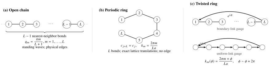
Open boundaries omit the wrapping bond and produce standing waves. Periodic boundaries close the graph and restore exact translations. A twist can be placed on one boundary link or distributed uniformly; both gauges have the same total loop phase and shifted momentum grid.

Momentum grid

A plane wave $c_j\sim e^{ikja}$ obeys the twist when

$$e^{ikLa} = e^{i\phi}.$$

Therefore

$$k_m(\phi) = \frac{2\pi m+\phi}{La}.$$

The twist shifts the sampled momenta through the same translation-invariant bulk dispersion. It does not generally change the continuous band function itself.

The unordered spectrum is $2\pi$ periodic:

$$\operatorname{Spec}H(\phi+2\pi) = \operatorname{Spec}H(\phi).$$

Individual eigenvalue branches can permute as $\phi$ advances by $2\pi$. This spectral flow contains physical information and should not be erased by relabeling too early.

Flux interpretation

For charge $q$ moving around a ring threaded by vector potential $\mathbf A$, the twist is the Aharonov–Bohm holonomy

$$\phi = \frac{q}{\hbar} \oint\mathbf A\cdot d\boldsymbol\ell \pmod{2\pi},$$

with sign fixed by charge and path orientation. A gauge transformation can move the vector potential into a boundary phase, but it cannot remove a nontrivial loop holonomy. Peierls Phase Preview develops the lattice gauge principle and plaquette fluxes.

Twists for spins

For a spin chain with conserved total $S^z$, a $U(1)$ spin twist can be defined by

$$s_{L+1}^{\pm} = e^{\pm i\phi}s_1^{\pm}, \qquad s_{L+1}^{z}=s_1^z.$$

The transverse exchange on the wrapping bond acquires conjugate phases while the longitudinal exchange does not. This probes spin stiffness rather than electric charge response.

Species-dependent twists

For spinful particles or several components, one may choose phases $\phi_\sigma$. Equal twists probe total charge motion. Opposite twists can probe spin or counterflow response. A calculation must state which conserved generator the twist couples to; the phrase twisted boundary conditions alone is incomplete.

Mode Grids at a Glance

For a uniform nearest-neighbor chain of $L$ sites, the common one-particle labels are:

Boundary	Identification or endpoint rule	Mode label	Exact translation sector?
open	no $(L,1)$ bond; fictitious $\psi_0=\psi_{L+1}=0$	$q_m=\pi m/(L+1)$, $m=1,\ldots,L$	no
periodic	$c_{j+L}=c_j$	$k_m=2\pi m/(La)$	yes
antiperiodic	$c_{j+L}=-c_j$	$k_m=(2m+1)\pi/(La)$	twisted translation
twisted	$c_{j+L}=e^{i\phi}c_j$	$k_m=(2\pi m+\phi)/(La)$	twisted translation

Every row contains exactly $L$ one-particle modes. Different integer ranges merely choose different representatives modulo the reciprocal-lattice period $2\pi/a$.

Do not mix denominators

The $L+1$ in the open standing-wave grid comes from the two fictitious nodes outside the physical chain. The $L$ in the periodic grid comes from winding around $L$ lattice spacings. Substituting one denominator for the other changes the finite Hamiltonian.

Momentum modulo a reciprocal vector

On a lattice,

$$k \sim k+\frac{2\pi}{a}.$$

A finite ring selects $L$ representatives from this equivalence class. The Brillouin-zone endpoint must not be counted twice.

Many-Body Momentum Sectors

For a periodic translation-invariant Hamiltonian, $T$ commutes with particle number, spin components preserved by the model, and the Hamiltonian. The Hilbert space decomposes as

$$\mathcal H = \bigoplus_K\mathcal H_K.$$

Exact diagonalization can work independently in each $K$ sector. This reduces matrix size and prevents unrelated symmetry blocks from contaminating level statistics.

Translation orbits of basis states

Let $|s\rangle$ be a product or occupation basis state. Its translation orbit is

$$\mathcal O_s = \{|s\rangle,T|s\rangle,\ldots,T^{r-1}|s\rangle\},$$

where $r$ is the smallest positive integer satisfying

$$T^r|s\rangle=|s\rangle.$$

A momentum-adapted combination is

$$|s;K\rangle \propto \sum_{n=0}^{r-1} e^{-iKn}T^n|s\rangle.$$

It is nonzero only when

$$e^{iKr}=1.$$

Basis states with shorter spatial period therefore contribute only to compatible momentum sectors. Ignoring this stabilizer condition produces zero vectors or incorrect normalization.

Total momentum for free modes

For independent periodic modes,

$$K_{\mathrm{tot}} = a\sum_k k n_k \pmod{2\pi}.$$

Interactions can mix occupation configurations while preserving their total $K_{\mathrm{tot}}$. Momentum conservation does not imply that individual particle momenta remain good quantum numbers.

Twisted translation

In a boundary-link gauge, ordinary translation moves the distinguished phased bond and may not visibly commute with the Hamiltonian. In a uniform-link gauge, all bonds carry the same phase and one-site translation is manifest. The two descriptions are unitarily equivalent; symmetry cannot depend on where a gauge places the phase.

For many particles, translating every particle around a twisted ring can accumulate a charge-dependent phase. State the translation operator and gauge convention before assigning momentum labels.

Open chains use other symmetries

An open uniform chain has no cyclic momentum sectors. It may have reflection parity,

$$R^2=I, \qquad [H_{\mathrm O},R]=0,$$

as well as internal symmetries such as particle number or total spin. Labeling an open-chain standing wave by $q_m$ is useful, but calling it an exact many-body momentum sector is misleading.

Fermion-Parity Caveat

Spatial periodicity for microscopic fermions and effective periodicity after a nonlocal spin transformation are different constructions.

Directly defined fermion ring

If the microscopic degrees of freedom are fermions on a ring, periodic, antiperiodic, or twisted spatial boundary conditions are independent model choices:

$$c_{L+1}=e^{i\phi}c_1.$$

No extra parity rule appears merely because the particles are fermions.

Fermions obtained from a periodic spin chain

For the Jordan–Wigner convention used in this volume, a periodic spin chain gives

$$c_{L+1} = -p c_1, \qquad p=(-1)^N.$$

Thus

Fermion parity $p$	Effective spatial fermion boundary	Mode grid
$+1$	antiperiodic	$k=(2m+1)\pi/(La)$
$-1$	periodic	$k=2\pi m/(La)$

The workflow is:

1. select a parity sector $p$;
2. impose the matching fermion boundary condition;
3. diagonalize the sector Hamiltonian;
4. retain only many-body states with physical parity $p$.

The boundary sign follows from the Jordan–Wigner string crossing the ordering cut. Jordan–Wigner Transformation gives the operator proof and treats the self-inverse $k=0$ and $k=\pi/a$ modes.

Pairing does not remove parity

A Bogoliubov Hamiltonian can violate particle-number conservation while preserving fermion parity. Its periodic and antiperiodic sectors must still be matched to the original spin sector. Diagonalizing both grids and keeping every quasiparticle state generally doubles the physical Hilbert space.

Spatial versus imaginary-time antiperiodicity

Spatial antiperiodic boundary conditions are a choice of finite geometry or flux. Fermionic fields in a thermal imaginary-time path integral are antiperiodic around the Euclidean-time circle because of the trace and Fermi statistics. These are different cycles and different statements. One does not imply the other.

Boundary Counting in Higher Dimensions

Consider a $d$-dimensional hyperrectangle with $L_\mu$ sites along direction $\mu$ and

$$V = \prod_{\mu=1}^{d}L_\mu$$

total sites. With open boundaries in every direction, the number of nearest-neighbor undirected bonds is

$$B_{\mathrm O} = \sum_{\mu=1}^{d} (L_\mu-1) \prod_{\nu\ne\mu}L_\nu.$$

With periodic boundaries in every direction and nondegenerate lengths,

$$B_{\mathrm P} = dV.$$

The missing-bond fraction scales like surface area divided by volume. For an isotropic $L^d$ sample,

$$\frac{B_{\mathrm P}-B_{\mathrm O}}{V} = \frac{d}{L}.$$

The formula assumes each periodic direction defines an ordinary cycle rather than a short multigraph. Very small $L_\mu$ again requires explicit edge counting.

Cylinder, torus, and slab

Boundary conditions may differ by direction:

• periodic in every direction gives a torus;
• periodic along one direction and open along another gives a cylinder;
• periodic in-plane and open transversely gives a slab;
• open in every direction gives a finite cluster with corners.

These geometries separate bulk, edge, hinge, and corner responses. A page or data file should list the choice in every primitive direction, not merely say mixed boundaries.

Twist vector

On a $d$-dimensional torus, assign a twist vector

$$\boldsymbol\phi = (\phi_1,\ldots,\phi_d).$$

The single-particle grid becomes

$$k_\mu = \frac{2\pi m_\mu+\phi_\mu}{L_\mu a_\mu}.$$

Each $\phi_\mu$ is a holonomy around a noncontractible cycle. It is distinct from the flux through an elementary plaquette, although both are represented by products of link phases.

Periodic images and long-range interactions

For short-range Hamiltonians, wrapping local bonds defines periodicity. For Coulomb, dipolar, or other long-range interactions, one must also specify how periodic images are summed. Minimum-image truncation, Ewald summation, and a direct finite-cluster interaction define different finite Hamiltonians. The words periodic boundary conditions do not settle this choice.

Bulk and Boundary Energy Scaling

For a one-dimensional local Hamiltonian with a well-defined bulk energy density $e_\infty$, typical large-$L$ forms are

$$E_{\mathrm O}(L) = Le_\infty +e_{\mathrm s} +\delta E_{\mathrm O}(L),$$ $$E_{\mathrm P}(L) = Le_\infty +\delta E_{\mathrm P}(L).$$

The open chain has an $O(1)$ surface energy $e_{\mathrm s}$. Dividing by $L$ makes this a $1/L$ correction to the energy density. The periodic chain has no physical surface term, but it still has finite-size corrections from quantized modes, virtual winding processes, and sector constraints.

Gapped systems

When a periodic system has a unique gapped bulk ground state and correlation length $\xi$, many local finite-size corrections are exponentially small,

$$\delta E_{\mathrm P}(L) \sim e^{-L/\xi},$$

up to prefactors and exceptions associated with topology, conserved sectors, or nearly degenerate vacua. Open systems can have $O(1)$ edge energies and exponentially small splittings between edge degrees of freedom.

Critical systems

A finite critical chain has a nonzero level spacing even though the thermodynamic gap vanishes. For a relativistic critical point with velocity $v$, the characteristic scale is

$$\Delta E(L) \sim \frac{v}{L}.$$

In conformal cases, periodic levels often have the form

$$E_n(L)-E_0(L) = \frac{2\pi v}{L}x_n +o(L^{-1}),$$

whereas open boundaries organize boundary scaling dimensions with a characteristic factor $\pi v/L$. The allowed $x_n$, degeneracies, and additive terms depend on the boundary and symmetry sector. A finite gap at one $L$ is therefore not evidence for a gapped phase.

Compare like with like

When comparing open and periodic total energies, first account for:

• the different number of bonds;
• surface fields or edge potentials;
• different allowed symmetry sectors;
• distinct shell fillings;
• whether the observable is total, per site, or per bond.

Bulk extrapolation should use intensive quantities and several sizes. Edge physics should be studied through boundary-local observables rather than divided away.

Shell Effects and Degeneracies

A finite periodic system samples a continuous dispersion at a discrete grid. Whether a sampled momentum lands exactly on a band crossing or Fermi point can change:

• ground-state degeneracy;
• the particle number of a closed shell;
• the apparent excitation gap;
• persistent current and stiffness estimates;
• which momentum sector contains the ground state.

Periodic and antiperiodic grids interlace. Comparing both is often more informative than treating either as uniquely correct for a bulk extrapolation.

Odd–even effects

Odd and even lengths can realize different graph properties. An even nearest-neighbor ring is bipartite; an odd ring is not. An antiferromagnetic Ising or Heisenberg interaction on an odd ring is geometrically frustrated because every bond cannot simultaneously realize the preferred staggered pattern.

Likewise, a periodic Ising ring has an even number of domain walls, while an open chain can contain a single wall. Such constraints can move the lowest state between sectors and change the first finite-size gap without changing the local bulk Hamiltonian.

Commensurability

Charge-density waves, spin spirals, and enlarged unit cells fit cleanly only when the finite dimensions are commensurate with their ordering wave vectors. An incompatible periodic cluster can force a defect or suppress an order parameter. Checking several cluster shapes is essential before concluding that an ordered phase is absent.

Flux Response and Stiffness

The dependence of the ground-state energy on a twist probes coherent transport around a ring. If physical flux $\Phi$ produces twist $\phi(\Phi)$, the persistent current is

$$I(\Phi) = -\frac{\partial E_0}{\partial\Phi}.$$

A charge or spin stiffness is proportional to the curvature

$$\mathcal D_L \propto L^{2-d} \left. \frac{\partial^2E_0} {\partial\phi^2} \right|_{\phi=0},$$

with prefactors depending on dimension, charge, lattice spacing, and Hamiltonian convention. State the convention before comparing numerical values.

An insulator is typically insensitive to a distant boundary twist in the thermodynamic limit, whereas a conductor or superfluid retains a finite stiffness. Finite-size level crossings, degeneracies, disorder averaging, and order of limits can complicate this diagnostic.

Twist averaging

Finite momentum-shell errors can be reduced by averaging an observable over twists:

$$\overline{O} = \frac{1}{(2\pi)^d} \int_0^{2\pi}d^d\phi\, O(\boldsymbol\phi).$$

In practice the integral is sampled on a finite twist grid. Twist averaging improves one-body momentum sampling and can smooth shell effects. It does not eliminate interaction finite-size errors, topological sector changes, or the need for size extrapolation.

Edges, Topology, and Entanglement

Open and periodic geometries answer different physical questions.

Edge states

A state localized near a termination can exist only when the relevant boundary is present. Its energy may lie in a bulk gap, and two opposite-edge modes can hybridize with a splitting

$$\Delta E_{\mathrm{edge}} \sim e^{-L/\xi_{\mathrm{edge}}}.$$

Closing the chain removes those physical edges. If the in-gap states disappear while the bulk bands remain, that is evidence for boundary localization, not a change in the bulk Hamiltonian.

Entanglement geometry

For a fixed interval length, periodic and open chains have different numbers of entanglement cuts. At a one-dimensional conformal critical point, this changes the logarithmic coefficient and boundary constants. The canonical entropy definitions and scaling caveats are on Entanglement Entropy in Many-Body Systems.

Bulk topology from twists

Periodic twists can probe bulk topology without introducing edges. In more than one dimension, adiabatic transport over a twist torus can define many-body polarization or Chern data under suitable gap and nondegeneracy assumptions. This is distinct from merely observing an edge state; bulk and boundary diagnostics should cross-check one another.

Boundary Choice by Method

Method or goal	Common boundary	Why it is useful	Main caveat
exact diagonalization	periodic or twisted	translation sectors reduce blocks; no surface	shell effects and cluster-shape dependence
edge-state spectroscopy	open	exposes physical terminations	bulk and edge levels coexist
DMRG or finite matrix-product states	open	lower entanglement and cheaper contractions	edge effects require central-window or scaling analysis
periodic matrix-product states	periodic	direct bulk ring and momentum comparison	greater computational cost at comparable accuracy
quantum Monte Carlo	periodic	reduces surface fraction; permits winding diagnostics	topology, sign, and ergodicity depend on representation
free-mode calculation	any	all choices are tractable one-body matrices	mode labels and degeneracies differ
Bethe ansatz	special periodic or open boundaries	preserves factorized structure in known cases	generic boundary fields or twists can break integrability
transport or stiffness	twisted periodic	differentiates energy with respect to flux	level crossings and prefactor conventions
thermodynamic bulk extrapolation	several choices	cross-checks finite-size bias	no single boundary removes all corrections

Why DMRG often starts open

Cutting a periodic ring into a linear tensor-network ordering introduces two entanglement cuts rather than one. For a fixed bond dimension, periodic calculations are therefore usually more demanding. Open calculations should measure bulk observables near the center and vary $L$ to separate edge profiles from bulk values.

Why exact diagonalization often starts periodic

Periodic boundaries remove physical edges and expose translation momentum. The Hilbert space is not smaller before symmetry resolution, but block diagonalization can reduce the largest matrix. Twists then scan momentum shells or probe response without changing the number of sites.

Exact solvability can depend on the boundary

An integrable bulk Hamiltonian does not make every boundary integrable. Periodic transfer matrices, reflection matrices for special open boundaries, and twisted transfer matrices obey different consistency conditions. Exact Solutions Preview gives the general integrability map; each model page states the boundary family for which its exact statements apply.

Implementation Checks

Construct bonds before operators

A robust finite-lattice implementation builds an explicit bond list

$$E = \{(i,j,\text{coupling data})\}$$

and validates it before assembling the Hamiltonian. Check:

• every site index is in range;
• each undirected bond appears once;
• directed reverse amplitudes are complex conjugates;
• open boundaries have no wrap bond;
• periodic directions have the expected bond count;
• twists multiply only the intended oriented crossings;
• short dimensions do not create accidental duplicate edges.

Fermion signs in an occupation basis

In a fixed Fock ordering, applying $c_i^\dagger c_j$ includes the parity of occupied modes between $i$ and $j$. Schematically,

$$c_i^\dagger c_j|\mathbf n\rangle \propto (-1)^{N_{(i,j)}} |\mathbf n'\rangle.$$

A wrapping hop is geometrically local on a ring but crosses the ordering cut in a linear bit representation. Its occupation-basis sign must still be evaluated correctly. This computational sign is part of the fermion algebra; it should not be replaced by an ad hoc constant boundary sign.

Hermiticity test

For every twist and sector, verify

$$\|H-H^\dagger\|=0$$

up to numerical tolerance. A missed conjugate on the wrapping hop is one of the most common sources of a non-Hermitian finite matrix.

Known-limit tests

At minimum, compare:

1. $\phi=0$ with the periodic Hamiltonian;
2. $\phi=\pi$ with the antiperiodic grid;
3. open and periodic bond counts;
4. a free model against analytical mode energies;
5. translation commutators in the chosen gauge;
6. $2\pi$ spectral periodicity as an unordered set;
7. Jordan–Wigner sector dimensions against the original spin Hilbert space.

Reading Finite-Size Data

Use a boundary condition as a diagnostic variable, not an invisible default. The broader Finite-Size Effects audit distinguishes boundary physics from quantization, shells, critical rounding, recurrence, and resolution; this section records the boundary-specific checks.

For a bulk phase

• compare several $L$ values at fixed density or other intensive control parameters;
• prefer periodic data for bulk translation symmetry, but inspect open data for edge contamination;
• compare periodic and antiperiodic shells when a Fermi point is involved;
• fit forms motivated by a gap, correlation length, or critical theory;
• vary cluster aspect ratio and commensurability in more than one dimension;
• distinguish total, surface, and bulk-normalized observables.

For edge physics

• use open geometry and resolve spatial profiles;
• increase the separation between opposite edges;
• compare with periodic geometry to identify states that require a boundary;
• perturb the edge locally without changing the bulk;
• test whether edge splittings decay exponentially or algebraically with size.

For transport

• record the twist convention and physical flux conversion;
• follow energy branches through level crossings rather than sorting only by energy;
• differentiate with a controlled step or fit around the chosen flux;
• resolve particle number, spin, and momentum sectors;
• test the order of $L\to\infty$, frequency $\omega\to0$, and temperature $T\to0$ limits.

Practical Boundary Checklist

Before trusting a finite-lattice result, record:

1. the site set and lattice dimensions;
2. every open, periodic, or twisted direction;
3. the oriented wrapping terms and their phases;
4. the number of sites, bonds, and local terms;
5. the gauge used to place each twist;
6. the exact symmetries that survive;
7. the momentum or reflection sectors retained;
8. any Jordan–Wigner parity projection;
9. the filling and whether the momentum shell is closed;
10. the observable normalization per site, bond, boundary length, or volume;
11. the finite-size sequence and aspect ratios;
12. the limiting procedure used to infer bulk behavior.

Common Mistakes

• Treating boundary conditions as a solver setting rather than part of the Hamiltonian.
• Calling an open lattice a periodic lattice with one weak bond without stating that perturbation.
• Setting the amplitude on the physical edge sites to zero instead of only the fictitious outside nodes.
• Using $2\pi m/L$ for open standing waves or $\pi m/(L+1)$ for periodic momentum.
• Calling an open-chain standing-wave label an exact translation momentum.
• Adding a wrapping bond twice through modulo indexing and a separate boundary term.
• Forgetting the conjugate phase on reverse hopping.
• Gauging away every link phase on a ring and losing the total holonomy.
• Assuming a $2\pi$ twist returns each labeled eigenbranch to itself rather than the spectrum as a set.
• Imposing the Jordan–Wigner parity rule on a directly defined fermion ring.
• Diagonalizing both Jordan–Wigner grids without projecting back to the matching parity sector.
• Confusing spatial antiperiodicity with thermal imaginary-time antiperiodicity.
• Comparing open and periodic total energies without correcting their bond counts.
• Interpreting a finite critical level spacing as a thermodynamic gap.
• Using one parity of $L$ or one cluster shape to infer a bulk phase.
• Expecting periodic boundaries to remove all finite-size effects.
• Using a periodic nearest-neighbor prescription for a long-range interaction without defining periodic images.

Exercises

Exercise 1: Count bonds on a rectangle

A square-lattice cluster has $L_x=4$ and $L_y=5$. Count nearest-neighbor undirected bonds for:

1. open boundaries in both directions;
2. periodic $x$ and open $y$ boundaries;
3. periodic boundaries in both directions.

Assume the dimensions are large enough that no short-cycle duplicate arises.

Solution

There are $V=L_xL_y=20$ sites. With both directions open,

$$B_{\mathrm{OO}} = (L_x-1)L_y + (L_y-1)L_x.$$

Therefore

$$B_{\mathrm{OO}} = 3\cdot5+4\cdot4 = 31.$$

Making $x$ periodic adds one wrapping $x$ bond in each of the five rows:

$$B_{\mathrm{PO}} = L_xL_y + (L_y-1)L_x = 20+16 = 36.$$

On the torus, each site contributes one positively oriented bond in each of two directions:

$$B_{\mathrm{PP}} = 2V = 40.$$

Counting only positive directions avoids counting each undirected bond twice.

Exercise 2: Compare mode grids

List the dimensionless one-particle labels $ka$ for a six-site uniform chain with periodic and antiperiodic boundaries. Give the open-chain standing-wave labels $q_m$.

Solution

For periodic boundaries, choose six representatives:

$$ka \in \left\{ 0, \pm\frac{\pi}{3}, \pm\frac{2\pi}{3}, \pi \right\}.$$

The points $\pi$ and $-\pi$ are equivalent, so only one is included.

For antiperiodic boundaries,

$$ka \in \left\{ \pm\frac{\pi}{6}, \pm\frac{\pi}{2}, \pm\frac{5\pi}{6} \right\}.$$

The open standing-wave labels are

$$q_m = \frac{\pi m}{7}, \qquad m=1,\ldots,6.$$

There are six modes in every case. Only the periodic and antiperiodic sets are translation-momentum grids.

Exercise 3: Move a twist between gauges

Begin with $c_{j+L}=e^{i\phi}c_j$ and define

$$c_j=e^{ij\phi/L}d_j.$$

Show that $d_j$ is periodic and that every forward hopping $c_j^\dagger c_{j+1}$ acquires the same phase.

Solution

Using the twisted condition,

$$e^{i(j+L)\phi/L}d_{j+L} = e^{i\phi}e^{ij\phi/L}d_j.$$

The phases on both sides are equal, so

$$d_{j+L}=d_j.$$

For one forward hop,

$$c_j^\dagger c_{j+1} = e^{-ij\phi/L}d_j^\dagger e^{i(j+1)\phi/L}d_{j+1},$$

hence

$$c_j^\dagger c_{j+1} = e^{i\phi/L}d_j^\dagger d_{j+1}.$$

Multiplying the $L$ forward-link phases gives $e^{i\phi}$. The boundary-link and uniform-link gauges therefore have the same loop holonomy.

Exercise 4: Translation-orbit compatibility

On a six-site periodic occupation chain, consider

$$|s\rangle=|100100\rangle.$$

Find its translation-orbit length and the momentum sectors to which its orbit can contribute.

Solution

Successive translations generate

$$|100100\rangle, \quad |010010\rangle, \quad |001001\rangle,$$

and the next translation returns to the first state. Thus $r=3$ even though the full chain has $L=6$.

A momentum projection is nonzero only if

$$e^{iKr}=1.$$

Therefore

$$K \in \left\{ 0, \frac{2\pi}{3}, \frac{4\pi}{3} \right\}.$$

These are all valid six-site lattice momenta because they correspond to $m=0,2,4$ in $K=2\pi m/6$.

Exercise 5: Jordan–Wigner parity sectors

Using $c_{L+1}=-pc_1$ with $p=(-1)^N$, determine the effective spatial boundary condition for sectors with $N=4$ and $N=5$. Explain why the answer is not a universal rule for every fermion ring.

Solution

For $N=4$,

$$p=(-1)^4=+1,$$

so

$$c_{L+1}=-c_1.$$

The effective fermions are antiperiodic.

For $N=5$,

$$p=(-1)^5=-1,$$

so

$$c_{L+1}=c_1.$$

They are periodic. This relation originates from the Jordan–Wigner string crossing the cut of a periodic spin chain. A microscopic fermion ring has its spatial boundary condition specified directly and need not obey this parity assignment.

Exercise 6: Surface energy from bond counting

For a ferromagnetic Ising chain at zero field,

$$H = -J\sum_{\langle j,k\rangle}Z_jZ_k, \qquad J>0,$$

find the all-up energy for an open chain and a periodic ring. Compare the energy per site.

Solution

Every aligned bond contributes $-J$. The open chain has $L-1$ bonds, so

$$E_{\mathrm O} = -(L-1)J.$$

The periodic ring has $L$ bonds:

$$E_{\mathrm P} = -LJ.$$

Their energy densities are

$$\frac{E_{\mathrm O}}{L} = -J+\frac{J}{L},$$ $$\frac{E_{\mathrm P}}{L} = -J.$$

The missing open bond is an $O(1)$ surface contribution and an $O(1/L)$ correction to the energy per site.

Exercise 7: Spectral flow under a full twist

For a free nearest-neighbor ring,

$$\varepsilon_m(\phi) = -2t\cos \left( \frac{2\pi m+\phi}{L} \right),$$

show that increasing $\phi$ by $2\pi$ leaves the spectrum invariant as a set. Does each fixed-$m$ branch return to itself?

Solution

Evaluate

$$\varepsilon_m(\phi+2\pi) = -2t\cos \left( \frac{2\pi(m+1)+\phi}{L} \right).$$

Therefore

$$\varepsilon_m(\phi+2\pi) = \varepsilon_{m+1}(\phi).$$

The set of $L$ energies is unchanged because $m$ is defined modulo $L$. A branch followed with fixed label $m$ flows into its neighbor rather than necessarily returning to itself after one flux quantum. After $L$ such cycles the simple fixed-label branch returns.

Exercise 8: Frustration on an odd ring

Let classical Ising variables $z_j=\pm1$ have antiferromagnetic energy

$$E = J\sum_{\langle j,k\rangle}z_jz_k, \qquad J>0.$$

Find the minimum energy for an open chain and for an odd periodic ring. Count the ground states of the odd ring.

Solution

An antialigned bond contributes $-J$. On an open chain, all $L-1$ bonds can be antialigned:

$$E_{\mathrm O}^{\min} = -(L-1)J.$$

On an odd ring, alternating signs cannot close consistently. At least one of the $L$ bonds must be aligned. A minimum configuration has $L-1$ satisfied bonds and one frustrated bond, so

$$E_{\mathrm P}^{\min} = -(L-1)J+J = -(L-2)J.$$

The frustrated bond can occupy any of the $L$ positions, and a global spin flip gives a distinct configuration. The ground-state degeneracy is therefore

$$2L.$$

The extensive bulk energy density still approaches $-J$, but the odd periodic topology enforces an $O(1)$ defect.

Key Takeaways

• A lattice boundary condition specifies graph closure, wrapping operators, phases, and sectors as part of the finite Hamiltonian.
• Open chains have physical edges and $L-1$ nearest-neighbor bonds; periodic rings have no edge and $L$ bonds.
• Open standing-wave labels are not exact translation momenta.
• A twist shifts the periodic momentum grid and is characterized by a gauge-invariant loop holonomy.
• Antiperiodic spatial boundaries are the special twist $\phi=\pi$ and are unrelated to thermal imaginary-time antiperiodicity.
• Direct fermion rings have independently chosen spatial boundaries; Jordan–Wigner fermions inherit parity-dependent boundaries from a periodic spin chain.
• Periodic boundaries remove surface terms but not shell effects, sector constraints, or critical finite-size gaps.
• Odd sizes, cluster shapes, and commensurability can force defects that mimic or obscure bulk behavior.
• Open, periodic, and twisted calculations answer complementary questions and should often be compared.

Further Reading on This Site

• Spin-$1/2$ Chain Model Dossier for the shared spin normalization, short-ring bond audit, symmetry sectors, and finite-chain benchmark handoffs.
• Tight-Binding Model for explicit open, periodic, and twisted one-particle diagonalization.
• Spinless Fermion Chains for shell filling, stiffness, and boundary parity in the interacting $t$–$V$ chain.
• Jordan–Wigner Transformation for the full parity-string derivation.
• Transverse-Field Ising Model for domain-wall parity, edge modes, and critical finite-size structure.
• XXZ Spin Chain for Bethe sectors and boundary-sensitive exact data.
• Translations and Momentum for the symmetry meaning of lattice momentum.
• Thermodynamic Limit for bulk, surface, and fixed-density limiting procedures.

References

1. E. Lieb, T. Schultz, and D. Mattis, “Two Soluble Models of an Antiferromagnetic Chain”, Annals of Physics 16, 407–466 (1961).
2. N. Byers and C. N. Yang, “Theoretical Considerations Concerning Quantized Magnetic Flux in Superconducting Cylinders”, Physical Review Letters 7, 46–49 (1961).
3. W. Kohn, “Theory of the Insulating State”, Physical Review 133, A171–A181 (1964).
4. M. E. Fisher and M. N. Barber, “Scaling Theory for Finite-Size Effects in the Critical Region”, Physical Review Letters 28, 1516–1519 (1972).
5. Q. Niu, D. J. Thouless, and Y.-S. Wu, “Quantized Hall Conductance as a Topological Invariant”, Physical Review B 31, 3372–3377 (1985).
6. B. S. Shastry and B. Sutherland, “Twisted Boundary Conditions and Effective Mass in Heisenberg–Ising and Hubbard Rings”, Physical Review Letters 65, 243–246 (1990).
7. S. R. White, “Density Matrix Formulation for Quantum Renormalization Groups”, Physical Review Letters 69, 2863–2866 (1992).
8. R. Resta, “Quantum-Mechanical Position Operator in Extended Systems”, Physical Review Letters 80, 1800–1803 (1998).
9. M. Oshikawa, “Commensurability, Excitation Gap, and Topology in Quantum Many-Particle Systems on a Periodic Lattice”, Physical Review Letters 84, 1535–1538 (2000).
10. C. Lin, F. H. Zong, and D. M. Ceperley, “Twist-Averaged Boundary Conditions in Continuum Quantum Monte Carlo Algorithms”, Physical Review E 64, 016702 (2001).