Entanglement Entropy in Many-Body Systems

Entanglement entropy turns a bipartite quantum-information definition into a structural probe of many-body states. The definition is simple: choose a subsystem $A$, trace out its complement $\bar A$, and compute the von Neumann entropy of the reduced state. The many-body content lies in how that entropy depends on the size and shape of $A$, the system size, the Hamiltonian parameters, the energy density, and the short-distance regulator.

For a pure many-body state $\lvert\Psi\rangle$ and a factorization

$$\mathcal H \cong \mathcal H_A\otimes\mathcal H_{\bar A},$$

the spatial entanglement entropy is

$$\begin{aligned} \rho_A &= \operatorname{Tr}_{\bar A} \lvert\Psi\rangle\langle\Psi\rvert, \\ S_A &= -\operatorname{Tr} \left( \rho_A\ln\rho_A \right). \end{aligned}$$

Natural logarithms are used throughout, so entropy is measured in nats. Divide by $\ln 2$ to express it in bits.

The canonical finite-dimensional definition and its information-theoretic properties belong to Entanglement Entropy. This page is the canonical home for many-body spatial entanglement: subsystem choices, exact benchmark states, area and volume laws, critical scaling, continuum qualifications, and consequences for numerical representation.

Canonical Scope

This page owns:

• entanglement across spatial, site, orbital, or mode partitions of many-body states;
• the dependence of $S_A$ and Rényi entropies on subsystem geometry and size;
• product-state, Bell-pair, GHZ, and typical-state benchmarks;
• area laws, logarithmic violations, and volume laws;
• one-dimensional conformal critical scaling;
• the relation between entropy growth and tensor-network bond dimension;
• practical finite-size, numerical, and experimental diagnostics.

Neighboring pages retain distinct ownership:

• Many-Body Entanglement Overview owns the chapter-level map among subsystem choices, global-state classes, information measures, and scaling limits.
• Entanglement Entropy owns the basic pure-state bipartite definition.
• Rényi Entropies owns the entropy family as a density-operator concept.
• Mutual Information owns the general information-theoretic definition of mutual information.
• Quantum Phase Transitions owns zero-temperature phase changes and their general finite-size scaling.
• Later pages in this chapter own area laws, volume laws, entanglement spectra, tensor networks, and entanglement at criticality. Topological Entanglement Entropy Preview owns the universal constant and its extraction protocols. The Many-Body Entanglement Glossary provides a compact cross-topic dictionary.

The Subsystem Is Part of the Question

Consider a lattice of $L$ sites with local Hilbert spaces $\mathcal H_j$. For distinguishable sites,

$$\mathcal H = \bigotimes_{j=1}^{L}\mathcal H_j.$$

A subset of sites $A$ defines

$$\mathcal H_A = \bigotimes_{j\in A}\mathcal H_j, \qquad \mathcal H_{\bar A} = \bigotimes_{j\notin A}\mathcal H_j.$$

Common choices include:

• one site against the rest;
• a contiguous block of $\ell$ sites in a chain;
• a half-system cut;
• a disk, strip, or rectangular region in higher dimensions;
• a set of orbitals, momentum modes, bands, or internal components.

These cuts are not interchangeable. A half-chain entropy probes a different organization of the state than a momentum-space partition. Even for the same state and the same number of degrees of freedom in $A$, changing the geometry can change the number of short-range bonds crossing the boundary and therefore change the leading entropy.

For a spatial region, denote its volume by $|A|$ and the size of its boundary by $|\partial A|$. On a lattice these may count sites and boundary links. In a continuum they carry dimensions and must be compared with a short-distance scale $a$.

Identical particles and constrained Hilbert spaces

For identical particles, particle labels do not usually define physical tensor factors. Site, orbital, mode, or spatial-region algebras are more appropriate. A Fock-space partition can often be defined from a chosen set of modes, but the answer then depends on that mode choice.

Gauge constraints create a sharper issue: the physical Hilbert space need not factorize into independent region Hilbert spaces because Gauss-law constraints couple boundary data. Extended-Hilbert-space constructions and algebraic definitions can produce related but not identical entropies. Any gauge-theory result must state the convention used. The simple tensor-product formula remains correct for ordinary spin and lattice-particle systems with a genuine regional factorization.

Reduced State and Schmidt Spectrum

For a pure state, the Schmidt decomposition across $A\vert\bar A$ is

$$\lvert\Psi\rangle = \sum_{\alpha=1}^{r} \sqrt{\lambda_\alpha}\, \lvert\alpha\rangle_A \lvert\alpha\rangle_{\bar A},$$

where

$$\lambda_\alpha\ge0, \qquad \sum_{\alpha=1}^{r}\lambda_\alpha=1.$$

The reduced states have the same nonzero eigenvalues:

$$\begin{aligned} \rho_A &= \sum_{\alpha=1}^{r} \lambda_\alpha \lvert\alpha\rangle_A \langle\alpha\rvert, \\ \rho_{\bar A} &= \sum_{\alpha=1}^{r} \lambda_\alpha \lvert\alpha\rangle_{\bar A} \langle\alpha\rvert. \end{aligned}$$

Therefore

$$S_A = S_{\bar A} = -\sum_{\alpha=1}^{r} \lambda_\alpha\ln\lambda_\alpha.$$

The equality $S_A=S_{\bar A}$ is a pure-state statement. It is useful in finite systems, where a block and its complement exchange roles under $\ell\mapsto L-\ell$.

The numbers $\lambda_\alpha$ form the entanglement spectrum in probability form. It is also common to define entanglement energies

$$\xi_\alpha = -\ln\lambda_\alpha,$$

up to an additive convention. Entanglement entropy compresses this entire spectrum to one number:

$$S_A = \sum_\alpha \lambda_\alpha\xi_\alpha.$$

If $d_A=\dim\mathcal H_A$, then

$$0 \le S_A \le \ln d_A.$$

The upper bound is attained when $\rho_A=I_A/d_A$, provided the complement is large enough to support that Schmidt rank.

Rényi Entropies for a Spatial Cut

The order-$n$ Rényi entropy is

$$S_A^{(n)} = \frac{1}{1-n} \ln\operatorname{Tr}(\rho_A^n), \qquad n>0, \quad n\ne1.$$

In terms of the Schmidt probabilities,

$$S_A^{(n)} = \frac{1}{1-n} \ln \left( \sum_\alpha\lambda_\alpha^n \right).$$

The von Neumann entropy is recovered by continuity:

$$S_A = \lim_{n\to1} S_A^{(n)}.$$

Different orders weight the entanglement spectrum differently. Large $n$ emphasizes its largest probability, while small positive $n$ is more sensitive to the number of populated Schmidt values. The second Rényi entropy,

$$S_A^{(2)} = -\ln\operatorname{Tr}(\rho_A^2),$$

is especially important in replica calculations, quantum Monte Carlo, and multi-copy experimental protocols.

Exact Benchmark States

Simple states prevent scaling terminology from becoming detached from the underlying reduced density matrix.

Product state

For

$$\lvert\Psi\rangle = \lvert\psi_A\rangle \otimes \lvert\phi_{\bar A}\rangle,$$

the reduced state is pure:

$$\rho_A = \lvert\psi_A\rangle\langle\psi_A\rvert.$$

Its spectrum is $(1,0,\ldots)$, so

$$S_A = S_A^{(n)} = 0.$$

A lattice product state therefore has zero entropy across every site partition. It is the simplest area-law state, with a vanishing area-law coefficient.

Independent Bell pairs

Suppose the state is a tensor product of Bell pairs and exactly $N_{\mathrm{cut}}$ pairs connect $A$ to $\bar A$. Each crossing pair contributes a maximally mixed qubit to $\rho_A$. Thus

$$\rho_A^{\mathrm{cut}} = \left( \frac{I_2}{2} \right)^{\otimes N_{\mathrm{cut}}},$$

and

$$S_A = N_{\mathrm{cut}}\ln2.$$

Every Rényi entropy gives the same value because all nonzero Schmidt probabilities are equal:

$$S_A^{(n)} = N_{\mathrm{cut}}\ln2.$$

This example gives the microscopic picture behind a short-range area law: only entangled pairs crossing the boundary contribute. A generic interacting ground state is not literally a product of Bell pairs, but finite-range entanglement leads to a similar boundary-dominated pattern.

GHZ state

For $L$ qubits, define

$$\lvert\mathrm{GHZ}_L\rangle = \frac{ \lvert0\rangle^{\otimes L} + \lvert1\rangle^{\otimes L} }{\sqrt2}.$$

For any nonempty proper subset $A$,

$$\rho_A = \frac12 \lvert0\rangle_A\langle0\rvert + \frac12 \lvert1\rangle_A\langle1\rvert,$$

so

$$S_A = S_A^{(n)} = \ln2.$$

The entropy is nonzero but independent of $|A|$. This illustrates two cautions: nonzero entanglement entropy need not imply a volume law, and a single entropy value does not uniquely characterize multipartite entanglement.

Typical states in a large Hilbert space

Let

$$\dim\mathcal H_A=m, \qquad \dim\mathcal H_{\bar A}=n, \qquad m\le n.$$

For a Haar-random pure state, Page’s result gives the mean subsystem entropy

$$\left\langle S_A\right\rangle = \sum_{k=n+1}^{mn} \frac1k - \frac{m-1}{2n}.$$

When $n$ is much larger than $m$,

$$\left\langle S_A\right\rangle = \ln m - \frac{m^2-1}{2mn} + \mathcal O\!\left(n^{-2}\right), \qquad \text{for fixed }m.$$

The reduced state is nearly maximally mixed, and the entropy is nearly the largest allowed by $\mathcal H_A$. If $m$ grows exponentially with the number of sites in $A$, this is a volume law. Typical vectors in Hilbert space are therefore far more entangled than low-energy states of many local gapped Hamiltonians.

Scaling with Region Size

The phrase entanglement scaling refers to a controlled family of regions and system sizes, not to a single entropy value. A scaling claim must specify:

• spatial dimension and lattice or continuum setting;
• the family of regions $A$;
• boundary conditions and total system size;
• whether the state is a ground state, excited eigenstate, time-evolved state, or mixed state;
• the order of the limits $L\to\infty$, $|A|\to\infty$, and regulator removal;
• whether the logarithm base and ultraviolet cutoff are fixed.

For a block of length $\ell$ in a chain, three common qualitative behaviors are shown below.

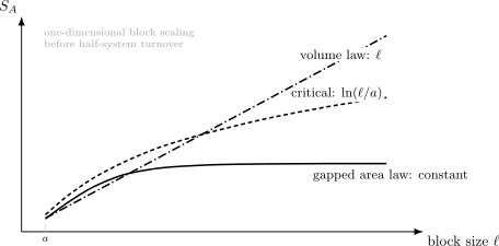
Schematic one-dimensional block scaling. A gapped area-law state saturates once $\ell$ exceeds its correlation length, a conformal critical ground state grows logarithmically, and a volume-law state grows linearly before finite-size symmetry under $\ell\leftrightarrow L-\ell$ becomes important. The curves are qualitative, not universal fits.

Area-Law Behavior

An area law means that the leading entropy of a large region scales with the size of its boundary rather than its volume:

$$S_A = \alpha \frac{|\partial A|}{a^{d-1}} + \text{subleading terms}.$$

Here $a$ is a microscopic length or ultraviolet cutoff. The coefficient $\alpha$ is generally nonuniversal: it depends on short-distance physics, the regulator, and the shape of the boundary.

In one spatial dimension, a connected interval has only a fixed number of boundary points. An area law therefore means that $S_A$ approaches a constant as the interval becomes large:

$$S_A(\ell) \longrightarrow S_\infty \qquad \text{for } \ell\gg\xi,$$

where $\xi$ is a finite correlation length.

For ground states of one-dimensional local Hamiltonians with a nonzero spectral gap, an area law can be established under standard locality and finite-dimensionality assumptions. This is a strong theorem, not merely a numerical pattern. In higher dimensions, area-law behavior is widely realized by gapped local phases, but no single unrestricted theorem covers every interacting Hamiltonian and every type of low-energy state. Area Laws gives the precise boundary conventions, theorem ledger, higher-dimensional status, and tensor-network caveats.

An area law is also not synonymous with triviality. Symmetry-protected and topologically ordered states can obey an area law while carrying nontrivial subleading data or entanglement-spectrum structure.

Critical Chains and Logarithmic Growth

At a one-dimensional quantum critical point described by a conformal field theory, interval entropy grows logarithmically. For a periodic chain of circumference $L$ and an interval of length $\ell$,

Luttinger Liquid Preview identifies the common $c=1$ compact-boson realization and explains why central charge counts modes while the Luttinger parameter controls continuously varying operator exponents.

$$S_A(\ell,L) = \frac{c}{3} \ln \left[ \frac{L}{\pi a} \sin \left( \frac{\pi\ell}{L} \right) \right] + s_1.$$

The central charge $c$ is universal, while the additive constant $s_1$ depends on microscopic details and on the cutoff convention. In the infinite-chain limit with $a\ll\ell\ll L$,

$$S_A(\ell) = \frac{c}{3} \ln\left(\frac{\ell}{a}\right) + s_1.$$

For an interval attached to the end of an open chain, the leading coefficient is halved:

$$S_A(\ell) = \frac{c}{6} \ln\left(\frac{\ell}{a}\right) + \widetilde s_1 + \cdots.$$

The periodic finite-size Rényi result is

$$S_A^{(n)}(\ell,L) = \frac{c}{6} \left( 1+\frac1n \right) \ln \left[ \frac{L}{\pi a} \sin \left( \frac{\pi\ell}{L} \right) \right] + s_n.$$

Taking $n\to1$ recovers the coefficient $c/3$. These formulas provide a practical route to estimating $c$, but finite-size corrections, boundaries, marginal operators, oscillatory terms, and an uncertain critical coupling can bias a fit.

The logarithm is an area-law violation in one dimension because a strict one-dimensional area law would be constant. It does not imply a volume law.

Fermi Surfaces and Logarithmic Area-Law Violations

Gapless fermions with an extended Fermi surface can violate the ordinary area law more strongly than an isolated relativistic critical point. For a smooth region of linear size $R$ in spatial dimension $d>1$, the leading behavior often has the form

$$S_A \sim \kappa\, R^{d-1} \ln\left(\frac{R}{a}\right).$$

The coefficient $\kappa$ depends on the geometry of both the real-space boundary and the Fermi surface. This scaling can be understood heuristically as contributions from many effectively one-dimensional gapless patches. The logarithmic enhancement is a diagnostic of codimension-one gapless structure, not a universal feature of every gapless phase.

Volume-Law Behavior

A volume law has leading scaling

$$S_A = s_{\mathrm{ent}}|A| + o(|A|),$$

for regions smaller than their complements. Typical random pure states and many highly excited eigenstates of nonintegrable systems display this behavior.

For a finite pure state,

$$S_A = S_{\bar A},$$

so a naive linear law cannot continue past half the system. A useful finite-size expectation is instead

$$S_A \propto \min\left(|A|,|\bar A|\right)$$

away from boundary and conservation-law corrections.

In systems satisfying the eigenstate thermalization hypothesis, the leading entropy density of a sufficiently small subsystem in a highly excited pure eigenstate can agree with the thermodynamic entropy density at the corresponding energy. This agreement concerns the leading reduced-state behavior; it does not turn the globally pure state into a thermal density operator.

Volume-law entanglement also appears dynamically after global quenches. Its growth can make exact state-vector simulation and fixed-bond-dimension tensor-network evolution impractical even while local observables remain simple.

Universal Subleading Information

The leading area term is often dominated by short-distance physics. Universal information may reside in subleading terms.

For suitable two-dimensional gapped topologically ordered phases and sufficiently smooth large regions,

$$S_A = \alpha\frac{|\partial A|}{a} - \gamma + \cdots,$$

where $\gamma$ is the topological entanglement entropy. Extracting $\gamma$ requires combinations of regions designed to cancel boundary contributions. Reading an intercept from a single small-region fit is generally unreliable.

Topological Order Preview connects this subleading term to anyon quantum dimensions, local indistinguishability, and noncontractible loop operators without making entropy alone a phase classifier.

Corners, Goldstone modes, Fermi surfaces, defects, and boundaries can produce additional logarithmic or constant terms. Their interpretation depends on geometry and universality class. The leading label “area law” does not determine the full expansion.

Continuum and Ultraviolet Dependence

In a continuum quantum field theory, arbitrarily short-wavelength modes straddle the entangling surface. The entropy of a sharply defined region is therefore generally ultraviolet divergent. Schematically,

$$S_A = c_{d-1} \frac{|\partial A|}{\epsilon^{d-1}} + c_{d-3} \frac{\mathcal G_2(\partial A)}{\epsilon^{d-3}} + \cdots,$$

where $\epsilon$ is a short-distance regulator and $\mathcal G_2(\partial A)$ denotes possible geometric contributions. The precise series depends on dimension, field content, regulator, and boundary geometry.

Consequently:

• the absolute entropy is not generally regulator independent;
• differences, derivatives, mutual information, and selected subleading terms can be better-defined observables;
• a lattice calculation includes an implicit ultraviolet cutoff;
• taking the continuum limit while holding a region fixed requires tracking the cutoff dependence.

The finite-dimensional formula is still the conceptual starting point, but continuum factorization and renormalization questions require additional care.

Pure-State Entanglement Versus Mixed-State Entropy

The reduced entropy $S_A$ is an entanglement measure across $A\vert\bar A$ only when the global state is pure. Entropy in Quantum Statistical Mechanics owns the broader comparison with equilibrium, diagonal, and coarse-grained entropies. If the many-body state is thermal,

$$\rho_\beta = \frac{e^{-\beta H}}{Z},$$

then

$$\rho_A = \operatorname{Tr}_{\bar A}\rho_\beta$$

is mixed because of both thermal uncertainty and correlations with $\bar A$. Its entropy can contain an extensive thermodynamic contribution:

$$S(\rho_A) = s_{\mathrm{th}}|A| + \text{boundary and finite-size terms}.$$

This volume term is not, by itself, bipartite entanglement. Mixed-state correlation and entanglement can instead be probed with mutual information, relative entropy, negativity, entanglement of formation, or other quantities chosen for the question at hand.

The distinction also matters for a pure excited eigenstate. The full state has zero von Neumann entropy,

$$S(\lvert E\rangle\langle E\rvert)=0,$$

while a subsystem can have volume-law entanglement entropy. Thermodynamic behavior of the subsystem emerges from entanglement with its complement, not from a mixed global ensemble.

Entanglement and Ordinary Correlations

Entanglement entropy and two-point correlation functions contain different information. Exponential decay of connected local correlations is compatible with nonzero area-law entanglement, and some states with unusual multipartite entanglement have deceptively simple two-point functions.

For a pure product state, all cross-cut correlations factorize and $S_A=0$. The converse is more nuanced in mixed states: classical correlations can make subsystem entropies and mutual information nonzero without entanglement.

Near a one-dimensional conformal critical point, both power-law correlations and logarithmic entanglement growth arise from the same long-distance theory. Away from such controlled settings, one should not infer an entropy scaling law from a single correlator.

Consequences for Tensor Networks

Variational Many-Body States gives the MPS coefficient formula and compares its entanglement bias with reference-based and neural ansätze. This section owns the entropy consequence of the bond dimension.

Across any cut, a matrix product state with bond dimension $\chi$ has Schmidt rank at most $\chi$. Therefore

$$S_A \le \ln\chi.$$

Equivalently, representing a state with entropy $S_A$ exactly requires

$$\chi \ge e^{S_A}.$$

This gives immediate scaling intuition:

• a one-dimensional area-law state can often be approximated with a bond dimension that does not grow exponentially with system size;
• a critical state with $S_A\sim(c/3)\ln\ell$ requires bond dimension growing polynomially with $\ell$ for controlled accuracy;
• a volume-law state requires bond dimension exponential in subsystem size for an exact generic representation.

The entropy bound is necessary but not sufficient for an efficient approximation. The detailed decay of Schmidt values, the desired observable accuracy, long-range structure, dimensionality, and algorithmic conditioning also matter. In higher dimensions, an area law alone does not guarantee a practical tensor-network contraction scheme.

Truncating an MPS bond keeps the largest Schmidt probabilities. If the discarded weight is

$$\varepsilon_{\mathrm{disc}} = \sum_{\alpha>\chi} \lambda_\alpha,$$

then the entanglement spectrum, not only $S_A$, controls the approximation error. Two states with equal entropy can have very different truncation behavior.

Computing Entanglement Entropy

Exact reduced density matrix

For a finite state vector, one may reshape its amplitudes into a matrix

$$\Psi_{i\mu},$$

where $i$ labels a basis of $A$ and $\mu$ labels a basis of $\bar A$. Then

$$(\rho_A)_{ij} = \sum_\mu \Psi_{i\mu} \Psi_{j\mu}^*.$$

A singular-value decomposition of $\Psi$ directly returns the Schmidt coefficients and avoids constructing both reduced density matrices. The cost still grows exponentially with subsystem size for a generic many-body vector.

Matrix product states

In a canonical MPS, the Schmidt probabilities across a bond are readily available. One computes

$$S_A = -\sum_\alpha \lambda_\alpha\ln\lambda_\alpha$$

without explicitly forming an exponentially large $\rho_A$. Block entropies away from a single bond can require additional contractions.

Free fermions

For a number-conserving fermionic Gaussian state, define the restricted correlation matrix

$$C_{ij} = \langle c_i^\dagger c_j\rangle, \qquad i,j\in A.$$

If its eigenvalues are $\nu_k\in[0,1]$, then

$$S_A = -\sum_k \left[ \nu_k\ln\nu_k + (1-\nu_k)\ln(1-\nu_k) \right].$$

The Rényi entropies are

$$S_A^{(n)} = \frac{1}{1-n} \sum_k \ln \left[ \nu_k^n + (1-\nu_k)^n \right].$$

This correlation-matrix method replaces a many-body density-matrix diagonalization with a one-particle matrix problem. Pairing states require the appropriate Nambu or Majorana covariance matrix, and bosonic Gaussian states use symplectic eigenvalues instead.

Replica and swap methods

For integer $n$,

$$\operatorname{Tr}(\rho_A^n)$$

can be represented using $n$ replicas cyclically joined along region $A$. In quantum Monte Carlo, this leads to swap-operator or replica-partition-function estimators. These methods can suffer from severe variance and free-energy-difference problems as the region grows.

Experimental Access

Entanglement entropy is nonlinear in the density operator, so it is not the expectation value of a single-copy observable. Full state tomography is exponentially costly for generic many-body systems.

Nevertheless, selected Rényi entropies and purities can be estimated through:

• interference between nominally identical copies;
• randomized local measurements and classical post-processing;
• swap operations in programmable quantum simulators;
• specialized protocols for Gaussian states or stabilizer states.

Every protocol relies on assumptions about state preparation, measurement fidelity, conserved sectors, and statistical sampling. A reported purity is meaningful only for the subsystem and ensemble actually reconstructed.

Finite-Size Analysis

A reliable scaling analysis should use more than a straight-line fit on a few sizes.

1. Specify the cut, geometry, boundary conditions, and state.
2. Compare $\ell$ with the lattice spacing $a$, correlation length $\xi$, and total size $L$.
3. Use the finite-size functional form appropriate to the proposed regime.
4. Exploit pure-state symmetry under $\ell\leftrightarrow L-\ell$ when applicable.
5. Fit several size windows and include plausible correction terms.
6. Check the same conclusion with Rényi entropies, spectra, correlations, or independent phase diagnostics.
7. Separate universal coefficients from nonuniversal additive and boundary terms.
8. State whether the thermodynamic, zero-temperature, and continuum limits commute in the calculation.

For a periodic critical chain, fitting $S_A$ against $\ln\ell$ while ignoring the chord length

$$d_L(\ell) = \frac{L}{\pi} \sin\left(\frac{\pi\ell}{L}\right)$$

can systematically bias the inferred central charge. The finite-size conformal formula uses $\ln[d_L(\ell)/a]$.

Physical Interpretation

Entanglement entropy answers a precise question: how mixed is the reduced state because degrees of freedom outside the chosen subsystem have been discarded from a pure global state?

Its most useful many-body interpretations are comparative:

• Does the entropy remain boundary dominated or become extensive?
• Does a universal coefficient identify a critical theory?
• Does the entropy change sharply or smoothly across a parameter sweep?
• Can a low-bond-dimension state represent the wavefunction accurately?
• Do subleading terms reveal topology, corners, boundaries, or gapless modes?
• How quickly does entanglement spread after a quench?

Entropy alone rarely identifies a phase. It should be combined with symmetry, correlations, excitation gaps, response functions, and, where relevant, topological invariants.

Common Mistakes

• Calling $S(\rho_A)$ an entanglement measure without checking that the global state is pure.
• Reporting an entropy without specifying the subsystem, geometry, boundary conditions, or logarithm base.
• Treating every gapped state in every dimension as covered by the one-dimensional area-law theorem.
• Calling logarithmic critical growth a volume law.
• Fitting the infinite-chain formula to a finite periodic chain without using the chord length.
• Inferring topological entanglement entropy from the intercept of one small-region fit.
• Ignoring ultraviolet dependence in a continuum calculation.
• Partitioning identical particles by unphysical particle labels.
• Assuming an area law alone guarantees an efficient higher-dimensional tensor-network algorithm.
• Comparing entropies from different conserved sectors or regulators as though they used the same Hilbert-space factorization.
• Interpreting entropy growth after a quench as proof that local observables have thermalized.
• Forgetting that $S_A=S_{\bar A}$ requires a pure global state.

Cross-Links

• Entanglement Spectrum — the full reduced-state eigenvalue data beyond one entropy.

• Mutual Information in Many-Body Systems — entropy combinations that isolate shared correlation and cancel independent bulk terms.

• Volume Laws

• Tensor Networks Preview — how virtual-bond cuts turn Schmidt-rank and entropy bounds into representation-capacity diagnostics.

• Matrix Product States Preview — canonical Schmidt bonds, the bound $S\le\ln\chi$, transfer spectra, and finite-entanglement convergence.

• Entanglement and Criticality — geometry-correct central-charge estimators, transition drift, and finite-size versus finite-entanglement inference.

• Many-Body and Quantum Statistical Mechanics

• Entanglement Entropy

• Rényi Entropies

• Schmidt Decomposition

• Mutual Information

• Entropy in Quantum Statistical Mechanics

• Thermal Entropy vs Entanglement Entropy

• Product States

• Bell States

• Entanglement in Many-Body Physics

• Correlation Functions Overview

• Quantum Phase Transitions

• Transverse-Field Ising Model

• XXZ Spin Chain

• Thermodynamic Limit

• Time-Dependent Variational Principle

• Ising Chain

• Many-Particle Hamiltonians

• Entanglement in QFT Preview

References

1. M. Srednicki, “Entropy and Area”, Physical Review Letters 71, 666–669 (1993).
2. C. Holzhey, F. Larsen, and F. Wilczek, “Geometric and Renormalized Entropy in Conformal Field Theory”, Nuclear Physics B 424, 443–467 (1994).
3. D. N. Page, “Average Entropy of a Subsystem”, Physical Review Letters 71, 1291–1294 (1993).
4. G. Vidal, J. I. Latorre, E. Rico, and A. Kitaev, “Entanglement in Quantum Critical Phenomena”, Physical Review Letters 90, 227902 (2003).
5. P. Calabrese and J. Cardy, “Entanglement Entropy and Quantum Field Theory”, Journal of Statistical Mechanics P06002 (2004).
6. M. B. Hastings, “An Area Law for One-Dimensional Quantum Systems”, Journal of Statistical Mechanics P08024 (2007).
7. D. Gioev and I. Klich, “Entanglement Entropy of Fermions in Any Dimension and the Widom Conjecture”, Physical Review Letters 96, 100503 (2006).
8. A. Kitaev and J. Preskill, “Topological Entanglement Entropy”, Physical Review Letters 96, 110404 (2006).
9. M. Levin and X.-G. Wen, “Detecting Topological Order in a Ground State Wave Function”, Physical Review Letters 96, 110405 (2006).
10. H. Li and F. D. M. Haldane, “Entanglement Spectrum as a Generalization of Entanglement Entropy”, Physical Review Letters 101, 010504 (2008).
11. L. Amico, R. Fazio, A. Osterloh, and V. Vedral, “Entanglement in Many-Body Systems”, Reviews of Modern Physics 80, 517–576 (2008).
12. J. Eisert, M. Cramer, and M. B. Plenio, “Area Laws for the Entanglement Entropy”, Reviews of Modern Physics 82, 277–306 (2010).
13. U. Schollwöck, “The Density-Matrix Renormalization Group in the Age of Matrix Product States”, Annals of Physics 326, 96–192 (2011).
14. P. Calabrese, J. Cardy, and B. Doyon, eds., Entanglement Entropy in Extended Quantum Systems, selected review material in Journal of Statistical Mechanics (2009).

Exercises

1. Product states and crossing Bell pairs. A spin chain is in a tensor product of single-site states except for three Bell pairs. Two Bell pairs cross the boundary of a chosen region $A$, while the third lies entirely inside $A$. Find $S_A$ and $S_A^{(n)}$.

Solution

Single-site product factors contribute no cross-boundary entanglement. A Bell pair lying entirely inside $A$ is part of a pure factor of $\rho_A$ and also contributes no entropy across the chosen cut.

Each of the two crossing Bell pairs contributes a reduced state $I_2/2$. Therefore

$$\rho_A \cong \left( \frac{I_2}{2} \right)^{\otimes2} \otimes \lvert\phi_A\rangle\langle\phi_A\rvert.$$

Its four nonzero eigenvalues are all $1/4$, so

$$S_A = -4\left(\frac14\right)\ln\left(\frac14\right) = 2\ln2.$$

For every positive Rényi order,

$$\begin{aligned} S_A^{(n)} &= \frac{1}{1-n} \ln \left[ 4\left(\frac14\right)^n \right] \\ &= 2\ln2. \end{aligned}$$

2. GHZ block entropy. Trace an $L$-qubit GHZ state over the complement of a nonempty proper subset $A$. Explain why the answer does not grow with $|A|$.

Solution

The density operator contains two diagonal branches and two off-diagonal coherences. Because $\bar A$ is nonempty,

$${}_{\bar A}\langle0\cdots0 \vert 1\cdots1\rangle_{\bar A} = 0,$$

so tracing out $\bar A$ removes the off-diagonal terms. The result is

$$\rho_A = \frac12 \lvert0\cdots0\rangle \langle0\cdots0\rvert + \frac12 \lvert1\cdots1\rangle \langle1\cdots1\rvert.$$

Its only nonzero eigenvalues are $1/2$ and $1/2$. Hence

$$S_A = \ln2.$$

The cut distinguishes only two globally correlated branches, independent of the number of qubits in $A$. The state has multipartite entanglement, but not a volume-law block entropy.

3. Rényi limit and a flat spectrum. Suppose $\rho_A$ has rank $r$ and all nonzero eigenvalues equal to $1/r$. Compute $S_A^{(n)}$ and verify its $n\to1$ limit.

Solution

The moment is

$$\operatorname{Tr}(\rho_A^n) = r\left(\frac1r\right)^n = r^{1-n}.$$

Therefore

$$S_A^{(n)} = \frac{1}{1-n} \ln r^{1-n} = \ln r.$$

It is independent of $n$, so the limit is immediate:

$$\lim_{n\to1} S_A^{(n)} = \ln r.$$

Directly, the von Neumann entropy gives

$$S_A = -r\left(\frac1r\right) \ln\left(\frac1r\right) = \ln r.$$

4. Extracting a central charge. In a periodic critical chain with $a\ll\ell_1,\ell_2\ll L$, the measured entropies are $S(\ell_1)$ and $S(\ell_2)$. Derive an estimator for the central charge that eliminates the nonuniversal additive constant.

Solution

Use the finite-size conformal form

$$S(\ell) = \frac{c}{3} \ln \left[ \frac{L}{\pi a} \sin\left(\frac{\pi\ell}{L}\right) \right] + s_1.$$

Subtracting the two entropies cancels both $s_1$ and the common factor $L/(\pi a)$:

$$S(\ell_2)-S(\ell_1) = \frac{c}{3} \ln \left[ \frac{ \sin(\pi\ell_2/L) }{ \sin(\pi\ell_1/L) } \right].$$

Thus

$$c_{\mathrm{est}} = 3\, \frac{ S(\ell_2)-S(\ell_1) }{ \ln \left[ \sin(\pi\ell_2/L)/ \sin(\pi\ell_1/L) \right] }.$$

In practice one should fit many block sizes and include corrections rather than rely on two points.

5. Distinguishing scaling regimes. For hypercubic regions of linear size $R$ in $d$ dimensions, compare the leading dependence expected for an area law, a Fermi-surface logarithmic violation, and a volume law.

Solution

The region volume and boundary scale as

$$|A| \propto R^d, \qquad |\partial A| \propto R^{d-1}.$$

An area law gives

$$S_A \propto R^{d-1}.$$

A codimension-one Fermi surface can produce

$$S_A \propto R^{d-1}\ln R.$$

A volume law gives

$$S_A \propto R^d.$$

The powers distinguish the leading regimes asymptotically. On small systems, subleading terms can make all three difficult to separate, so geometry and multiple sizes are essential.

6. Bond dimension requirement. A family of half-chain entropies scales as

$$S(L) = \frac{c}{6}\ln L + s_0$$

for an open critical chain. Find the minimum scaling of an exact MPS bond dimension implied by entropy alone. Contrast it with a volume law $S(L)=sL/2$.

Solution

Because an MPS of bond dimension $\chi$ satisfies

$$S \le \ln\chi,$$

an exact representation must obey

$$\chi \ge e^S.$$

For the critical chain,

$$\chi \ge e^{s_0} L^{c/6}.$$

Entropy alone therefore requires at least polynomial growth with $L$. This is a lower bound, not a guarantee that the stated bond dimension achieves a desired approximation error.

For the volume law,

$$\chi \ge \exp\left(\frac{sL}{2}\right),$$

which is exponential in system size. This explains why generic volume-law states are incompatible with efficient fixed-bond-dimension MPS representations.