Many-Body Entanglement Overview

Many-body entanglement is the organization of quantum correlations across a specified split of a system with many degrees of freedom. The finite-system definition does not change: choose accessible observables or a subsystem $A$, form its reduced state, and inspect how strongly that state fails to be pure or factorized from its complement. What changes in many-body physics is the question being asked.

A useful statement must specify at least four ingredients:

$$\begin{gathered} \text{subsystem or observable split}, \\ \text{global state and state class}, \\ \text{information measure}, \\ \text{scaling limit and control variables}. \end{gathered}$$

Without those ingredients, phrases such as “highly entangled,” “area-law state,” or “thermal entanglement” are incomplete. A state can be weakly entangled across a real-space cut and strongly entangled across a momentum-space cut. A subsystem entropy can diagnose pure-state entanglement, mixed-state uncertainty, or both. A finite-size curve can look linear before crossing over to saturation.

The central many-body question is therefore not merely

$$\text{Is the state entangled?}$$

It is

$$\begin{gathered} \text{How is quantum information distributed} \\ \text{across scale, geometry, modes,} \\ \text{energy density, and time?} \end{gathered}$$

Scope and Canonical Ownership

This page owns the chapter-level framework:

• how a tensor factorization or observable algebra defines the entanglement question;
• the distinction among spatial, site, mode, orbital, species, and particle partitions;
• reduced density matrices as complete local states;
• the transition from a single finite bipartition to a controlled family of subsystem sizes and system sizes;
• the taxonomy of boundary-law, logarithmic, and volume-law behavior;
• how state class, purity, temperature, energy density, and dynamics change the interpretation;
• how entanglement data complement correlation functions, order parameters, spectra, and response;
• a decision workflow for selecting a measure and checking whether a scaling claim is controlled.

Neighboring pages retain narrower canonical homes:

• Tensor Products of Hilbert Spaces owns the finite-system tensor-product construction.
• Reduced Density Operators and Partial Trace own the general marginal-state definition and calculation.
• Entanglement Depends on a Decomposition owns the finite-system proof that entanglement is relative to a chosen subsystem structure.
• Schmidt Decomposition owns the finite-dimensional theorem and singular-value construction.
• Entanglement Entropy owns the basic pure-state bipartite measure.
• Entanglement Entropy in Many-Body Systems owns detailed spatial entropy formulas, Rényi scaling, benchmark states, area and volume laws, critical-chain fits, and numerical extraction.
• Mutual Information owns the general total-correlation measure for mixed states.
• Mode Decompositions owns the construction and basis dependence of field and oscillator modes.
• Identical-Particle Entanglement Cautions owns operational distinctions among particle slots, modes, regions, and superselection constraints.
• Entropy in Quantum Statistical Mechanics owns thermodynamic entropy and ensemble identities.

The purpose here is orientation with enough mathematics to prevent category errors. It is not a duplicate derivation of every entropy formula that later pages specialize. The Many-Body Entanglement Glossary is the compact companion for notation, identities, scaling forms, and assumption checks.

Convention Ledger

Logarithms and units

Unless a base is displayed explicitly, use natural logarithms:

$$S(\rho) := -\operatorname{Tr} \left( \rho\ln\rho \right).$$

Entropy is then measured in nats. Entropy in bits is

$$S_2(\rho) = \frac{S(\rho)}{\ln2}.$$

Changing the logarithm base changes numerical units, not the ordering of states by entropy.

Region and complement

Write $A$ for the chosen subsystem and $\bar A$ for its complement. For a genuine tensor factorization,

$$\mathcal H \cong \mathcal H_A \otimes \mathcal H_{\bar A}.$$

The reduced state is

$$\rho_A := \operatorname{Tr}_{\bar A}\rho.$$

For spatial regions, $|A|$ denotes region volume or number of sites, while $|\partial A|$ denotes boundary measure or the number of cut links. These are distinct geometric quantities.

Pure and mixed global states

A pure global state is written

$$\rho = \lvert\Psi\rangle\langle\Psi\rvert, \qquad \rho^2=\rho.$$

A mixed global state obeys

$$\rho^2\ne\rho$$

unless it happens to be pure. The same reduced-state entropy has different interpretations in these two cases.

Scaling variables

Separate subsystem size $\ell$, total linear size $L$, short-distance cutoff $a$, correlation length $\xi$, inverse temperature $\beta$, and evolution time $t$. A scaling claim should state which variables are held fixed and the order in which limits are taken:

$$\ell,\ L,\ \xi,\ \beta,\ t,\ a.$$

For example, $\ell\to\infty$ at fixed finite $L$ is not a thermodynamic scaling limit.

Entanglement Requires a Subsystem Question

Observable meaning before algebra

The reduced state $\rho_A$ is not defined by circling coefficients in a wavefunction. It is defined by the collection of measurements assigned to $A$. In a tensor-product system, every local observable has the form

$$O_A\otimes I_{\bar A},$$

and $\rho_A$ is characterized by

$$\operatorname{Tr}_{\mathcal H} \left[ \rho \left( O_A\otimes I_{\bar A} \right) \right] = \operatorname{Tr}_{\mathcal H_A} \left( \rho_A O_A \right)$$

for every $O_A$. Thus $\rho_A$ is the complete state seen by an observer restricted to the chosen local algebra.

This operational statement remains useful when a simple tensor factorization becomes subtle. The first question is always: which observables can the putative subsystem access?

The same vector can answer different questions

Let a finite Hilbert space admit two decompositions,

$$\mathcal H \cong \mathcal H_A\otimes\mathcal H_{\bar A} \cong \mathcal H_C\otimes\mathcal H_{\bar C}.$$

A vector can be product across one split and entangled across the other:

$$\lvert\Psi\rangle = \lvert\psi\rangle_A \otimes \lvert\phi\rangle_{\bar A},$$

while

$$\operatorname{rank} \rho_C > 1.$$

Entanglement is therefore not a scalar property of a ket without additional structure. The Hamiltonian, geometry, locality, preparation, and measurement protocol usually select physically useful structures, but the selection must be stated.

Common Many-Body Partitions

Lattice sites and spatial regions

For a spin or finite-local-dimension lattice,

$$\mathcal H = \bigotimes_{j=1}^{N} \mathcal H_j.$$

A set of sites $A$ gives the natural factorization

$$\mathcal H_A = \bigotimes_{j\in A}\mathcal H_j, \qquad \mathcal H_{\bar A} = \bigotimes_{j\notin A}\mathcal H_j.$$

Useful geometries include:

• a single site;
• a contiguous interval in one dimension;
• a half-chain or half-cylinder;
• a disk, strip, annulus, or rectangle;
• two separated regions used to form mutual information;
• a checkerboard or sublattice partition.

Geometry matters. Two regions with the same $|A|$ may have very different $|\partial A|$, corner content, connectivity, and topology.

Spatial regions in particle and field systems

For particles on a real-space lattice, site orbitals supply local factors. In a continuum field theory, the physically robust object is more fundamentally the algebra of observables supported in a region. Formally one often writes

$$\mathcal H \overset{?}{\cong} \mathcal H_A \otimes \mathcal H_{\bar A},$$

but the question mark matters. Arbitrarily short-distance correlations make continuum spatial entropy regulator dependent, and local relativistic algebras do not behave like ordinary finite-dimensional tensor factors.

A lattice spacing or ultraviolet cutoff $a$ supplies a regulated definition. Claims about continuum universality must isolate cutoff-independent combinations, coefficients, or differences rather than treating the full entropy as finite.

Mode and orbital partitions

Choose orthonormal one-particle modes labeled by $i$. Their occupation degrees of freedom generate a Fock-space description. A subset $\mathcal I_A$ of modes defines a mode partition:

$$\mathcal I = \mathcal I_A \sqcup \mathcal I_{\bar A}.$$

Examples include:

• left and right localized orbitals;
• positive and negative momenta;
• momentum patches near different Fermi-surface regions;
• bands, valleys, layers, or sublattices;
• spin-up and spin-down modes;
• frequency bins or wavepacket modes.

A unitary change of one-particle basis,

$$\widetilde c_\alpha = \sum_i U_{\alpha i}c_i,$$

can change mode entanglement because it changes the subsystem definition. Real-space and momentum-space partitions are therefore not competing estimates of one invariant quantity. They probe different organizations of the state.

Species, layer, and internal-component partitions

In multicomponent systems one may place different species, layers, bands, or internal states on opposite sides of a split:

$$\mathcal H \cong \mathcal H_{\mathrm{species}\ 1} \otimes \mathcal H_{\mathrm{species}\ 2}.$$

This can diagnose interspecies pairing, spin-charge organization, layer coherence, or hybridization. It does not directly measure spatial short-range entanglement.

Particle partitions and identical particles

For distinguishable particles, labeled particle Hilbert spaces can define physical subsystems. For identical bosons or fermions, formal slots in

$$\mathfrak h^{\otimes N}$$

are not independently addressable particles. The physical fixed-number spaces are

$$\operatorname{Sym}^N\mathfrak h, \qquad \bigwedge^N\mathfrak h.$$

Exchange-required nonfactorization in slot labels should not automatically be counted as an operational entanglement resource. Region or mode partitions are usually clearer. When a particle partition is used, state the convention, accessible operations, and any number-superselection restriction.

Constrained and gauge-invariant systems

Local constraints can prevent the physical Hilbert space from factorizing across a boundary. Schematically,

$$\mathcal H_{\mathrm{phys}} \ne \mathcal H_{A,\mathrm{phys}} \otimes \mathcal H_{\bar A,\mathrm{phys}}.$$

Gauss-law constraints are the standard example: electric flux through the boundary is shared data. Algebraic definitions, center choices, and extended-Hilbert-space constructions can assign different boundary contributions while agreeing on appropriate universal information.

The practical rule is simple: never import the unconstrained partial-trace formula into a gauge or constrained system without stating how boundary degrees of freedom are treated.

The Reduced State Is the Local Information

Partial trace for a genuine factorization

Choose bases $\{\lvert a\rangle\}$ and $\{\lvert b\rangle\}$ for $A$ and $\bar A$. For

$$\rho = \sum_{a,a',b,b'} \rho_{ab,a'b'} \lvert a,b\rangle \langle a',b'\rvert,$$

the reduced matrix has entries

$$\left( \rho_A \right)_{aa'} = \sum_b \rho_{ab,a'b}.$$

The operation discards inaccessible labels but preserves every local expectation value. It does not describe a physical measurement unless a measurement protocol is separately specified.

Pure-state Schmidt data

For a finite pure bipartition,

$$\lvert\Psi\rangle = \sum_{\alpha=1}^{\chi} \lambda_\alpha \lvert\alpha\rangle_A \lvert\alpha\rangle_{\bar A},$$

where

$$\lambda_\alpha>0, \qquad \sum_\alpha\lambda_\alpha^2=1.$$

The nonzero reduced-state eigenvalues are

$$p_\alpha = \lambda_\alpha^2.$$

Consequently,

$$\operatorname{spec}_{\ne0}\rho_A = \operatorname{spec}_{\ne0}\rho_{\bar A},$$

and every spectral entropy agrees across the cut:

$$S_A=S_{\bar A}.$$

This equality is a pure-state statement. It generally fails for a mixed global state.

Local mixedness has two possible origins

If the global state is pure, local mixedness is entirely due to entanglement with the complement. If the global state is mixed, $\rho_A$ can be mixed because of:

• entanglement across the $A\vert\bar A$ split;
• classical correlations;
• global statistical uncertainty;
• coupling to an omitted environment;
• coarse graining or an ensemble average.

Thus

$$S(\rho_A)$$

is not by itself a mixed-state entanglement measure. A thermal product state can have extensive subsystem entropy and no entanglement between its sites.

Choose the Information Object

Von Neumann and Rényi entropies

The von Neumann entropy is

$$S_A = -\operatorname{Tr} \left( \rho_A\ln\rho_A \right).$$

The Rényi family is

$$S_A^{(n)} := \frac{1}{1-n} \ln \operatorname{Tr} \rho_A^n, \qquad n>0, \quad n\ne1.$$

When the limit exists,

$$\lim_{n\to1}S_A^{(n)} = S_A.$$

Different $n$ weight the entanglement spectrum differently. Large $n$ emphasizes its largest eigenvalues; small $n$ is more sensitive to broad support.

Spectrum and entanglement Hamiltonian

Writing

$$\rho_A = \frac{e^{-K_A}} {\operatorname{Tr}e^{-K_A}}$$

defines an entanglement or modular Hamiltonian $K_A$, up to an additive constant. If

$$\rho_A = \sum_\alpha p_\alpha \lvert\alpha\rangle\langle\alpha\rvert,$$

then entanglement energies may be defined by

$$\xi_\alpha := -\ln p_\alpha$$

up to a common shift convention. The spectrum contains more information than any one entropy, but its physical interpretation remains partition dependent.

Mutual information

For a state on two regions $A$ and $B$,

$$I(A:B) := S_A+S_B-S_{AB}.$$

It measures total correlation, not entanglement alone. It is useful for mixed states and separated regions because local ultraviolet boundary terms can cancel in the combination. It obeys

$$I(A:B)\ge0,$$

with equality exactly for

$$\rho_{AB} = \rho_A\otimes\rho_B.$$

Negativity and other mixed-state probes

Mixed-state entanglement generally requires information beyond $S_A$. The logarithmic negativity,

$$\mathcal E_N := \ln \left\| \rho_{AB}^{T_B} \right\|_1,$$

is one computable option, with qualifications for fermions and continuum systems. Entanglement witnesses, operational resource measures, and multipartite invariants answer still different questions.

No single scalar orders all many-body states by “amount of entanglement.”

Operator entanglement

An operator can be mapped to a vector in a doubled Hilbert space after choosing an inner product and normalization. Its entanglement then probes operator complexity, channel structure, or growth under dynamics. This is distinct from state entanglement:

$$\lvert\Psi(t)\rangle \quad\text{versus}\quad O(t).$$

The distinction becomes important in scrambling, matrix-product-operator simulation, and open-system evolution. Operator Entanglement and Scrambling Preview owns the normalization, operator Schmidt spectrum, simulation-cost, and information-spreading ledger.

From One Bipartition to a Scaling Law

A controlled family of questions

A single value $S_A$ is a property of one state and one split. A many-body scaling statement compares a family:

$$S_A = S \left( \ell,L,\xi,\beta,t,a; \text{shape, boundary conditions, state} \right).$$

To claim asymptotic behavior, vary enough of these parameters to distinguish leading growth from constants and crossover corrections.

For a pure state on a finite system,

$$S(\ell,L) = S(L-\ell,L)$$

for complementary intervals when the geometry identifies them. A fit that violates this symmetry has likely mixed conventions, boundary conditions, or numerical errors.

Boundary, logarithmic, and volume growth

In a local system with spatial region $A$, three common leading behaviors are:

$$\begin{aligned} \text{boundary law:} \qquad S_A &\sim \alpha |\partial A|, \\ \text{logarithmic enhancement:} \qquad S_A &\sim \alpha |\partial A| \ln(\ell/a), \\ \text{volume law:} \qquad S_A &\sim s |A|. \end{aligned}$$

In one dimension, a connected interval has a boundary of fixed size. A boundary law therefore appears as saturation:

$$S_A \longrightarrow \text{constant}$$

when $\ell$ exceeds the correlation length in a suitable gapped ground state.

At a one-dimensional conformal critical point, one instead often finds

$$S_A \sim \frac{c}{3} \ln(\ell/a) +\text{constant}$$

for one interval in an infinite periodic setting. The coefficient changes with boundaries, geometry, and Rényi index. The detailed formulas belong to the spatial entropy page.

A taxonomy, not a universal trichotomy

Leading behavior	Common setting	What it suggests	What it does not prove
$S_A=0$	exact product across the chosen cut	no entanglement across that cut	product across every other partition
$S_A=O(1)$ in 1D	many gapped local ground states	boundary-law structure	trivial phase or short-range entanglement in every sense
$S_A\sim\ln\ell$	many 1D critical ground states	scale-invariant low-energy structure	a volume law or a unique universality class
$S_A\sim	\partial A	\ln\ell$	systems with extended Fermi surfaces
$S_A\sim	A	$	typical states, thermalizing eigenstates, late quenches

Long-range interactions, disorder, constraints, fracton-like structures, non-Hermitian settings, and special excited states can require other classifications.

Benchmark State Families

State family	Reduced spectrum across the stated cut	Entanglement lesson
Product state	one eigenvalue equal to one	zero for that partition, not necessarily every repartition
$n_\partial$ independent Bell pairs crossing the cut	$2^{n_\partial}$ equal eigenvalues	$S_A=n_\partial\ln2$ gives a literal boundary-counting model
GHZ or cat state	two equal nonzero eigenvalues for any proper nonempty site subset	$S_A=\ln2$ is global branch information, not one pair per boundary link
Flat Schmidt spectrum of rank $r$	$p_i=1/r$	$S_A=\ln r$ and exact bond dimension at least $r$
Typical pure state with $\dim\mathcal H_A\ll\dim\mathcal H_{\bar A}$	close to maximally mixed on $A$	near-volume-law entropy can arise in a globally pure state

The table is a diagnostic ledger; the subsections below explain the qualifications and scaling limits.

Product state

For

$$\lvert\Psi_{\mathrm{prod}}\rangle = \bigotimes_{j=1}^{N} \lvert\phi_j\rangle,$$

every site partition has

$$\rho_A = \lvert\phi_A\rangle \langle\phi_A\rvert, \qquad S_A=0.$$

This does not imply zero entanglement in every mode basis. A nonlocal mode transformation can redefine the tensor factors.

Independent pairs crossing a boundary

Suppose $m_{\partial}$ maximally entangled pairs cross the boundary and all remaining factors lie entirely within $A$ or $\bar A$. Then

$$\rho_A \cong \left( \frac{I_q}{q} \right)^{\otimes m_{\partial}} \otimes \lvert\phi_A\rangle \langle\phi_A\rvert$$

for local pair dimension $q$. Therefore

$$S_A = m_{\partial}\ln q.$$

Short-range entanglement localized near a boundary gives the simplest microscopic picture of a boundary law.

Cat and GHZ states

For

$$\lvert\mathrm{GHZ}_N\rangle = \frac{ \lvert0\rangle^{\otimes N} + \lvert1\rangle^{\otimes N} }{\sqrt2},$$

every nontrivial proper site subset has two equal reduced-state eigenvalues:

$$\operatorname{spec}_{\ne0}\rho_A = \left\{ \frac12,\frac12 \right\}.$$

Hence

$$S_A=\ln2,$$

independent of subsystem volume. Long-range correlation does not require volume-law entanglement.

Fixed-number delocalized states

For the one-excitation state

$$\lvert W_N\rangle = \frac{1}{\sqrt N} \sum_{j=1}^{N} \lvert0\cdots1_j\cdots0\rangle,$$

a region of $\ell$ sites has nonzero reduced-state eigenvalues

$$\frac{\ell}{N}, \qquad 1-\frac{\ell}{N}.$$

Thus

$$S_A = h_2 \left( \frac{\ell}{N} \right),$$

where

$$h_2(x) := -x\ln x -(1-x)\ln(1-x).$$

The answer depends on the subsystem fraction $\ell/N$, not on a boundary or volume coefficient.

Typical highly excited pure states

For a random pure state in

$$\mathcal H_A\otimes\mathcal H_{\bar A}, \qquad d_A\le d_{\bar A},$$

the smaller subsystem is typically close to maximally mixed:

$$S_A \approx \ln d_A -\text{small correction}.$$

If $d_A$ grows exponentially with $|A|$, this is a volume law. This statement is about typical vectors in a chosen Hilbert-space measure, not about every eigenstate of a local Hamiltonian.

Thermal mixed states

A Gibbs state

$$\rho_\beta = \frac{e^{-\beta H}}{Z}$$

can have extensive $S(\rho_A)$ because $\rho_\beta$ is globally mixed. That extensive entropy is not automatically entanglement between $A$ and $\bar A$. Mutual information or a mixed-state entanglement measure is needed to separate correlation questions.

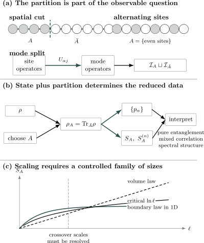
Three layers of a many-body entanglement claim. First choose physical subsystems: the same lattice may be divided by a spatial cut, by alternating sites, or by a nonlocal mode transformation. Next reduce the global state to $\rho_A$ and decide whether its spectrum is being used as pure-state entanglement data, mixed-state correlation data, or an entanglement spectrum. Only then compare a controlled family of sizes: one-dimensional boundary-law saturation, critical logarithmic growth, and volume-law growth are distinct asymptotic classes, not labels inferred from one finite point.

What Entanglement Reveals Physically

Information not visible in one-point data

Two states can have the same local expectation values and different global organization. For example, a product state and an entangled state may both satisfy

$$\langle S_j^z\rangle=0$$

at every site. Reduced spectra can distinguish how local mixedness is embedded in the full wavefunction.

This makes entanglement useful when no simple local order parameter is available. It does not make ordinary observables obsolete. Energy gaps, symmetry quantum numbers, correlation functions, response, and boundary conditions remain necessary context.

Correlation and entanglement are related but not equivalent

For bounded operators $O_A$ and $O_B$ supported on disjoint regions, quantum mutual information controls connected correlations through inequalities of the schematic form

$$\frac{ \left| \langle O_AO_B\rangle - \langle O_A\rangle \langle O_B\rangle \right|^2 }{ 2 \|O_A\|^2 \|O_B\|^2 } \le I(A:B),$$

with logarithm and normalization conventions understood. Thus small mutual information forces all bounded connected correlations to be small.

The converse is weaker. A short list of two-point functions does not determine a many-body reduced state. Multipartite or topological organization can remain invisible to selected low-order correlators.

Ground-state phases

Within a gapped local phase, the leading boundary-law coefficient is usually nonuniversal and sensitive to the microscopic cutoff. More robust information can live in:

• symmetry-resolved patterns;
• protected degeneracies in an entanglement spectrum;
• universal corner or logarithmic coefficients;
• subleading topological terms;
• changes that cannot occur under a finite-depth local unitary preserving the relevant symmetry.

An area law alone does not distinguish a trivial product phase from every symmetry-protected, symmetry-broken, or topologically ordered phase.

Critical points

At a continuous quantum critical point, correlations extend across scales and spatial entropy often acquires universal logarithmic or shape-dependent information. In one dimension, conformal systems provide the best-known example:

$$S_A \propto c\ln\ell,$$

where the coefficient can reveal a central charge after geometry and boundary conventions are fixed.

Finite systems also contain oscillatory, marginal, boundary, and irrelevant-operator corrections. A visually straight line against $\ln\ell$ is evidence to test, not a self-validating central-charge measurement.

Topological order

In a suitable two-dimensional gapped state, a simply connected region may have

$$S_A = \alpha|\partial A| -\gamma +\cdots,$$

where $\gamma$ can encode total quantum dimension. Directly fitting an intercept is unreliable because corners, finite correlation length, symmetry breaking, and boundary details also contribute constants.

Region combinations designed to cancel local boundary terms provide the controlled construction. Topological Entanglement Entropy Preview owns those subtraction protocols and their limitations, while Topological Order Preview owns the phase-specific meaning.

Numerical complexity

Across one cut, an exact pure state with Schmidt rank $\chi$ can be written using $\chi$ matched terms:

$$\lvert\Psi\rangle = \sum_{\alpha=1}^{\chi} \lambda_\alpha \lvert\alpha\rangle_A \lvert\alpha\rangle_{\bar A}.$$

The entropy obeys

$$S_A \le \ln\chi.$$

Therefore a matrix product state with bond dimension $D$ satisfies

$$S_A \le \ln D$$

across that bond. Boundary-law structure helps explain why many one-dimensional ground states admit efficient tensor-network approximations, while volume-law dynamics drives rapid bond-dimension growth.

The inequality is one-way. A modest entropy does not by itself guarantee that a small-$D$ approximation reaches a requested error, and higher Rényi entropies or the tail of the Schmidt spectrum may matter.

Dynamics and information spreading

After a global quench, a state that begins with low spatial entanglement can develop growing entanglement as correlated excitations spread. In short-range systems, one often expects a causal or effective light-cone structure:

$$\ell_{\mathrm{corr}}(t) \lesssim v_{\mathrm{LR}}t,$$

where $v_{\mathrm{LR}}$ is a Lieb–Robinson-type velocity scale rather than necessarily a quasiparticle group velocity.

For a fixed cut, entropy can grow approximately linearly over an intermediate window:

$$S_A(t) \sim v_E s_{\mathrm{eq}}t,$$

before finite-size saturation. Integrable, localized, constrained, long-range, and monitored systems can exhibit different laws. Entanglement growth is therefore a dynamical diagnostic, not a universal clock.

Partition-Specific Interpretation

Real-space cuts

Real-space cuts are natural for local Hamiltonians because interactions couple nearby degrees of freedom. They expose:

• short-range boundary entanglement;
• critical scaling with distance;
• topological subleading terms;
• entanglement growth after local or global quenches;
• the bond-dimension cost of real-space tensor networks.

They are also the cuts most sensitive to ultraviolet regularization in continuum limits.

Momentum-space cuts

Momentum partitions can reveal pairing and scattering structure. A BCS-like state, for example, naturally correlates modes $\mathbf k$ and $-\mathbf k$. A partition that separates them can have strong mode entanglement even when a different orbital basis reorganizes the same state.

Because momentum modes are nonlocal in real space, momentum-space entropy need not obey a real-space boundary law. Its scaling should be interpreted using the geometry of the chosen momentum set, the dispersion, and interaction channels.

Orbital and band cuts

Orbital entanglement can diagnose hybridization among atomic orbitals, Landau-level orbitals, bands, or localized Wannier sectors. The answer depends on the orbital basis:

$$c_i \longmapsto \widetilde c_\alpha = \sum_i U_{\alpha i}c_i.$$

A basis chosen by symmetry, locality, experimental addressability, or a low-energy projection can make the partition physically meaningful. An arbitrary basis rotation can make the same numerical entropy hard to interpret.

Species and spin cuts

Separating spin components, particle species, layers, or valleys can quantify intercomponent organization. Such cuts may be useful in:

• paired superfluids;
• Kondo and impurity systems;
• bilayers;
• spin-orbit-coupled systems;
• multicomponent ultracold gases.

They should not be called spatial area laws unless a spatial region is also part of the definition.

Geometric versus internal boundaries

A region boundary is a boundary in physical space. A mode, species, or orbital split has an abstract boundary in the chosen factorization. Both define legitimate entanglement questions, but only the former supports statements such as

$$S_A\propto|\partial A|$$

with $\partial A$ a physical surface.

State Class Changes the Question

Ground states

For ground states of local Hamiltonians, entanglement reflects locality, the gap structure, low-energy fields, and phase organization. The important limits are often

$$L\to\infty, \qquad \ell\to\infty, \qquad \frac{\ell}{L} \ \text{controlled}.$$

One should compare states with matching boundary conditions and symmetry sectors.

Individual excited eigenstates

An excited eigenstate is still pure. Its subsystem entropy can be volume law even though the global entropy vanishes:

$$S(\rho)=0, \qquad S(\rho_A)>0.$$

In a thermalizing system, sufficiently small subsystems of typical finite-energy-density eigenstates can resemble thermal reduced states. This is a statement associated with the eigenstate thermalization hypothesis, not an identity between global thermodynamic entropy and pure-state entanglement.

Thermal states

A Gibbs state is mixed:

$$\rho_\beta = \frac{e^{-\beta H}} {\operatorname{Tr}e^{-\beta H}}.$$

Its subsystem entropy contains thermal uncertainty. For a large region,

$$S(\rho_{\beta,A}) \sim s_{\mathrm{th}}(\beta)|A| +\text{boundary corrections},$$

even when entanglement between $A$ and $\bar A$ is small. The forthcoming thermal-versus-entanglement page will own the full comparison; Entropy in Quantum Statistical Mechanics owns the ensemble entropy.

Nonequilibrium pure states

Unitary time evolution preserves global purity:

$$\rho(t) = U(t) \rho(0) U^\dagger(t).$$

Yet subsystem entropy can grow because information moves from local degrees of freedom into correlations:

$$S_A(t) = S_{\bar A}(t)$$

for a globally pure bipartition. This is not fundamental information loss.

Open and monitored systems

For a mixed state generated by noise, dissipation, or measurement averaging, subsystem entropy conflates entanglement with environmental and classical uncertainty. Conditional trajectories and the ensemble-averaged density operator can have very different entanglement.

Any claim about measurement-induced transitions or dissipative entanglement must specify whether it concerns:

• individual conditioned trajectories;
• an unconditioned mixed state;
• a purification including the environment;
• an experimentally accessible estimator.

Scaling-Limit Audit

Subsystem fraction

For a one-dimensional pure system of length $L$, compare results at fixed fraction

$$x := \frac{\ell}{L}$$

or explicitly work in

$$a\ll\ell\ll L.$$

Mixing small-$x$ and half-system data can hide finite-size curvature.

Boundary conditions

Open and periodic systems have different numbers of entanglement cuts. At criticality this changes logarithmic coefficients and boundary constants. A spatial interval touching an open edge is not equivalent to an interval embedded in a periodic chain.

Symmetry sectors

Finite systems may return a symmetry-preserving cat state where the thermodynamic phase is described by symmetry-broken pure states. A cat contribution can add an $O(1)$ entropy:

$$\Delta S_A \sim \ln g$$

for $g$ coherently superposed sectors. Whether to retain or remove it depends on the physical state preparation and limiting procedure.

Cutoff and local dimension

The leading boundary coefficient can depend on:

• lattice spacing;
• local Hilbert-space truncation;
• orbital basis;
• regulator;
• geometric discretization;
• how a curved boundary crosses lattice links.

Universal claims should use quantities protected against these changes.

Order of limits

The limits

$$L\to\infty, \qquad \ell\to\infty, \qquad a\to0, \qquad t\to\infty$$

need not commute. For example, finite-volume unitary dynamics has recurrences, while a thermodynamic limit can support irreversible-looking local relaxation.

Error bars and fit windows

Entropies derived from a numerical state inherit:

• truncation error;
• finite bond dimension;
• Monte Carlo uncertainty;
• analytic-continuation or tomography error;
• finite-size corrections;
• uncertainty from fitting an asymptotic form outside its regime.

Report fit-window variation and competing functional forms rather than only a covariance matrix from one favored fit.

Computing Many-Body Entanglement

Exact diagonalization and coefficient reshaping

For a pure state represented in a product basis,

$$\lvert\Psi\rangle = \sum_{a,b} C_{ab} \lvert a\rangle_A \lvert b\rangle_{\bar A},$$

reshape amplitudes into the matrix $C$. Then

$$\rho_A = CC^\dagger.$$

If

$$C = U\Lambda V^\dagger,$$

the diagonal entries $\lambda_\alpha$ of $\Lambda$ are Schmidt coefficients. One can compute

$$p_\alpha=\lambda_\alpha^2, \qquad S_A=-\sum_\alpha p_\alpha\ln p_\alpha$$

without explicitly forming a larger density matrix.

The basis ordering must match the intended subsystem split. A silent bit-ordering error can produce a normalized but physically wrong spectrum.

Symmetry-resolved blocks

If an additive conserved quantity decomposes as

$$Q = Q_A+Q_{\bar A},$$

then $\rho_A$ often block diagonalizes:

$$\rho_A = \bigoplus_q p_q \rho_{A,q}, \qquad \operatorname{Tr}\rho_{A,q}=1.$$

The entropy separates into number fluctuation and within-sector pieces:

$$S_A = -\sum_q p_q\ln p_q + \sum_q p_q S(\rho_{A,q}).$$

This decomposition is useful, but the two terms are not individually basis independent under operations that mix charge sectors.

Gaussian fermions

For a number-conserving fermionic Gaussian state, restrict the one-body correlation matrix to $A$:

$$\left( C_A \right)_{ij} := \langle c_i^\dagger c_j \rangle, \qquad i,j\in A.$$

If its eigenvalues are $\nu_m$, then

$$S_A = -\sum_m \left[ \nu_m\ln\nu_m + (1-\nu_m) \ln(1-\nu_m) \right].$$

Pairing states require the covariance or Nambu formulation. Interacting non-Gaussian states are not determined by the two-point matrix alone.

Matrix product states

At an MPS bond in canonical form, the stored Schmidt values directly give

$$S_A = -\sum_{\alpha=1}^{D} \lambda_\alpha^2 \ln\lambda_\alpha^2.$$

Useful diagnostics include:

• entropy convergence with bond dimension $D$;
• discarded weight;
• the tail of the Schmidt spectrum;
• dependence on sweep tolerance;
• finite-entanglement scaling near criticality.

An apparent entropy plateau can be physical saturation or a bond-dimension ceiling. Varying $D$ distinguishes them.

Quantum Monte Carlo and replica estimators

Rényi entropies can be expressed through replicated partition functions or swap operators. For the second Rényi entropy,

$$S_A^{(2)} = -\ln \operatorname{Tr} \rho_A^2.$$

In a two-copy construction, $\operatorname{Tr}\rho_A^2$ is the expectation of a swap on region $A$. The estimator can have severe variance or rare-event problems as region size grows, so ratio tricks and carefully designed sampling are often needed.

Experimental access

Experiments can access selected Rényi entropies, randomized-measurement estimators, purity, or lower bounds with multiple copies or statistical protocols. Any reported quantity must state:

• whether the global state is pure;
• which region or modes define $A$;
• the assumed symmetries or number sectors;
• bias correction and finite sampling;
• state-preparation and measurement errors;
• whether the estimator is an entropy, a witness, or a bound.

Full many-body tomography scales exponentially and is rarely the practical route.

Numerical error ledger

Before interpreting an entropy or entanglement spectrum, record four distinct error channels:

Channel	Audit
State preparation or solver error	norm, energy variance, residual, convergence with tolerance or sweep count
Subsystem construction	basis ordering, complement symmetry for pure states, conserved-sector weights
Spectrum processing	Hermiticity, $\operatorname{Tr}\rho_A=1$, positivity, discarded weight, cutoff sensitivity
Scaling inference	size and geometry variation, fit-window drift, competing asymptotic forms, covariance

Tiny negative eigenvalues can arise from roundoff. Blindly clipping them and renormalizing hides whether the error is harmless or structural. Report the most negative eigenvalue and trace defect, vary numerical precision, and show that the claimed quantity is stable under a justified positivity repair.

A Reliable Interpretation Workflow

1. Name the physical subsystem. State whether $A$ is a spatial region, a set of sites, modes, orbitals, species, or an observable algebra.
2. State the global-state class. Pure ground state, individual eigenstate, Gibbs state, quench state, open-system state, or measurement trajectory lead to different meanings.
3. Choose the information object. Entropy, Rényi entropy, mutual information, negativity, spectrum, or operator entanglement should match the question.
4. Fix units and conventions. Give the logarithm base, normalization, boundary conditions, and regulator.
5. Specify the scaling family. List $\ell$, $L$, $a$, $\xi$, $\beta$, $t$, and the order of limits.
6. Benchmark simple states. Product, crossing-pair, cat, and random-state limits catch normalization and partition errors.
7. Vary numerical controls. Increase size, bond dimension, sample count, local cutoff, or solver precision.
8. Fit competing asymptotics. Compare saturation, logarithmic, and linear growth with explicit correction terms.
9. Combine diagnostics. Check gaps, symmetry sectors, correlations, response, and known phase information.
10. Phrase only the demonstrated claim. A finite-size crossover is not an asymptotic law, and a subsystem entropy of a mixed state is not automatically entanglement.

Worked Checks

Check 1: purity bound

For a subsystem of dimension $d_A$,

$$0 \le S_A \le \ln d_A.$$

The lower bound is saturated by a pure reduced state. The upper bound is saturated by

$$\rho_A = \frac{I_A}{d_A}.$$

Any computed entropy outside this interval signals normalization, eigenvalue, logarithm, or roundoff trouble.

Check 2: complement symmetry

For a globally pure state,

$$S_A=S_{\bar A}.$$

In exact diagonalization, computing both sides is a strong reshaping test. A mismatch beyond numerical tolerance means the two coefficient matrices do not represent complementary cuts of the same normalized state.

Check 3: local-unitary invariance

For

$$\lvert\Psi'\rangle = \left( U_A\otimes U_{\bar A} \right) \lvert\Psi\rangle,$$

the reduced state transforms as

$$\rho_A' = U_A\rho_AU_A^\dagger.$$

Therefore its eigenvalues and all spectral entropies are unchanged. A code that changes $S_A$ under independent basis rotations within $A$ and $\bar A$ is not computing a basis-invariant reduced spectrum.

Check 4: a unitary across the cut

A two-site gate acting with one site in $A$ and one in $\bar A$ can change Schmidt values. For two qubits,

$$\lvert00\rangle \longmapsto \frac{ \lvert00\rangle+\lvert11\rangle }{\sqrt2}$$

changes

$$S_A:0\longmapsto\ln2.$$

The distinction between local gates and gates crossing the cut underlies circuit pictures of entanglement growth.

Check 5: mixed product state

Let

$$\rho_{AB} = \rho_A\otimes\rho_B$$

with both factors mixed. Then

$$S_A>0, \qquad S_B>0$$

can hold, while

$$I(A:B)=0.$$

This is the minimal counterexample to identifying local entropy with entanglement for a mixed global state.

Decision Table

Physical question	Natural subsystem	Useful first object	Essential caution
How complex is a 1D ground state for DMRG?	contiguous real-space cut	Schmidt spectrum and $S_A$	vary bond dimension and cut position
Is a critical chain consistent with a CFT?	intervals at several $\ell$ and $L$	Rényi or von Neumann scaling	include boundaries and correction terms
How correlated are separated thermal regions?	disjoint spatial regions	mutual information	it includes classical and quantum correlation
Is pairing organized between opposite momenta?	momentum-mode split	mode reduced state	basis and superselection dependence
Does a topological state contain edge-like entanglement structure?	phase-appropriate orbital or spatial cut	entanglement spectrum	finite-size counting is not a theorem of phase identity
Why does real-time MPS simulation fail?	every bond along the chain	entropy and discarded spectrum	distinguish physical growth from truncation saturation
Is a noisy mixed state entangled?	operational laboratories or modes	negativity, witness, or bound	subsystem entropy alone is insufficient
Is a continuum coefficient universal?	regulated spatial regions	cutoff-canceling combination	state the algebra, regulator, and boundary convention

Common Mistakes

Calling a ket entangled without naming a split

Always state the tensor factorization, mode choice, region algebra, or operational laboratories. The same vector can have different entanglement under different decompositions.

Treating identical-particle slots as laboratories

Required symmetrization or antisymmetrization does not by itself establish accessible entanglement. Use physical regions, modes, or explicitly defined particle operations.

Equating subsystem entropy with mixed-state entanglement

For mixed $\rho_{AB}$, $S_A$ includes local and classical uncertainty. Use a measure designed for the mixed-state question.

Inferring an asymptotic law from one size

Area, logarithmic, and volume behavior concern families of regions. At least one controlled scaling variable and meaningful correction analysis are required.

Ignoring geometry

Region volume, boundary size, number of components, corners, and topology can all affect entropy. Equal $|A|$ does not imply equal $S_A$.

Ignoring boundary conditions

Open and periodic chains have different cuts and critical coefficients. Do not combine them in one fit without an explicit formula.

Calling every area-law state trivial

Symmetry-protected, symmetry-broken, and topologically ordered states can all obey boundary laws. Leading scaling alone does not classify the phase.

Calling logarithmic growth a volume law

In one dimension,

$$\ln\ell \ll \ell$$

as $\ell\to\infty$. These growth classes have different physical and computational implications.

Reading an entanglement spectrum as a physical energy spectrum

Entanglement energies are derived from $\rho_A$. Their relation to a physical boundary Hamiltonian can be powerful but is not automatic or exact in every model.

Mistaking a bond-dimension ceiling for physical saturation

An MPS has

$$S_A\le\ln D.$$

If the observed plateau tracks $\ln D$, increase $D$ before claiming a boundary law.

Dropping the ultraviolet regulator

Continuum spatial entropy generally diverges. Universal statements concern selected coefficients or combinations, not the unregulated total.

Using entanglement as a stand-alone phase label

Entanglement should be combined with Hamiltonian symmetries, gaps, correlations, response, and finite-size spectra. One scalar entropy is rarely a complete classifier.

Exercises

1. Three partitions of four qubits. Consider

   $$\lvert\Psi\rangle = \frac{ \lvert0000\rangle + \lvert1111\rangle }{\sqrt2}.$$

   Compute the entropy for $A=\{1\}$, $A=\{1,2\}$, and $A=\{1,3\}$. Explain why the geometry does not matter for this state.

Solution

For every nonempty proper subset $A$, tracing out $\bar A$ removes the coherence between the all-zero and all-one branches because the complementary branch states are orthogonal. Thus

$$\rho_A = \frac12 \lvert0\cdots0\rangle \langle0\cdots0\rvert + \frac12 \lvert1\cdots1\rangle \langle1\cdots1\rvert.$$

Its nonzero spectrum is

$$\left\{ \frac12,\frac12 \right\},$$

so all three partitions give

$$S_A=\ln2.$$

The GHZ state stores one coherent global branch bit. It does not contain an independent entangled pair on every cut link, so changing the boundary geometry does not change this entropy.

2. Crossing-pair boundary law. A chain contains nearest-neighbor Bell pairs on bonds $(1,2),(3,4),\ldots$. Find the entropy of a contiguous interval for cuts that pass through zero, one, or two Bell pairs.

Solution

Bell pairs wholly inside $A$ or wholly inside $\bar A$ are pure factors relative to the bipartition and contribute no entropy. Each pair cut by the boundary contributes one maximally mixed qubit to $\rho_A$ and hence $\ln2$.

Therefore

$$S_A = m_{\partial}\ln2, \qquad m_{\partial}=0,1,2.$$

The result depends on the number of cut entangled bonds, not on the number of sites in the interval.

3. Pure versus thermal product states. Let

   $$\rho = \bigotimes_{j=1}^{N} \frac{ e^{-\beta h\sigma_j^z} }{ 2\cosh(\beta h) }.$$

   Find the entropy of a region of $\ell$ spins and the mutual information between that region and its complement. Is the volume-law region entropy entanglement?

Solution

One spin has probabilities

$$p_{\pm} = \frac{ e^{\mp\beta h} }{ 2\cosh(\beta h) }.$$

Its entropy is

$$s_1 = -p_+\ln p_+ -p_-\ln p_-.$$

Because the state is a tensor product,

$$S_A = \ell s_1.$$

However,

$$\rho = \rho_A\otimes\rho_{\bar A},$$

so

$$I(A:\bar A)=0.$$

The volume law is entirely thermal local mixedness, not entanglement across the cut.

4. Mode dependence of one particle. A single boson occupies

   $$\lvert\psi\rangle = \frac{ a_L^\dagger+a_R^\dagger }{\sqrt2} \lvert0\rangle.$$

   Compute the entropy for the $L\vert R$ mode split. Then define

   $$a_+^\dagger = \frac{ a_L^\dagger+a_R^\dagger }{\sqrt2}, \qquad a_-^\dagger = \frac{ a_L^\dagger-a_R^\dagger }{\sqrt2},$$

   and compute the entropy for the $+\vert-$ split.

Solution

In the $L,R$ occupation basis,

$$\lvert\psi\rangle = \frac{ \lvert1\rangle_L\lvert0\rangle_R + \lvert0\rangle_L\lvert1\rangle_R }{\sqrt2}.$$

The reduced $L$-mode spectrum is $\{1/2,1/2\}$, so

$$S_L=\ln2.$$

In the rotated basis,

$$\lvert\psi\rangle = a_+^\dagger\lvert0\rangle = \lvert1\rangle_+ \lvert0\rangle_-.$$

This is a product across the $+\vert-$ mode split:

$$S_+=0.$$

The state has not changed. The subsystem definition has.

5. Schmidt-rank and MPS bounds. A state has Schmidt coefficients

   $$\lambda_\alpha = \frac{1}{\sqrt\chi}, \qquad \alpha=1,\ldots,\chi.$$

   Find $S_A$ and the minimum exact MPS bond dimension across that cut.

Solution

The reduced-state eigenvalues are

$$p_\alpha = \lambda_\alpha^2 = \frac1\chi.$$

Therefore

$$S_A = -\chi \left( \frac1\chi \right) \ln \left( \frac1\chi \right) = \ln\chi.$$

An exact MPS representation must accommodate every nonzero Schmidt value, so its bond dimension satisfies

$$D\ge\chi.$$

The minimally sufficient exact value at that cut is $D=\chi$.

6. Complement-symmetry audit. A numerical calculation of a normalized pure state on ten qubits reports

   $$S_{\{1,2,3\}}=1.24, \qquad S_{\{4,\ldots,10\}}=1.31.$$

   What can be concluded before any physical interpretation?

Solution

The two listed regions are complementary. For a normalized pure state, their nonzero reduced spectra must agree exactly, so

$$S_{\{1,2,3\}} = S_{\{4,\ldots,10\}}.$$

The discrepancy means that at least one premise or implementation is wrong. Possibilities include:

• the state is actually mixed;
• the regions are not complementary under the code’s basis ordering;
• one reduced matrix is not normalized;
• different logarithm bases were used;
• numerical truncation is uncontrolled.

No phase or scaling claim should be made until this audit passes.

7. Distinguishing logarithmic and linear growth. Suppose data over $\ell=4,\ldots,16$ fit both

   $$S(\ell)=a+b\ln\ell$$

   and

   $$S(\ell)=a'+s\ell$$

   within the quoted pointwise errors. Give at least four additional checks needed before assigning a scaling class.

Solution

Useful checks include:

1. extend to larger $\ell$ and several total sizes $L$;
2. hold $\ell/L$ fixed or use a finite-size formula appropriate to the boundary conditions;
3. vary the fit window and include leading correction terms;
4. compare information criteria or held-out residuals for competing models;
5. verify convergence with bond dimension or solver tolerance;
6. check complement symmetry for a pure state;
7. inspect gaps and correlation-length estimates;
8. test open and periodic formulas separately.

Agreement on a short interval is not asymptotic evidence because $\ln\ell$ can look nearly linear over a narrow window.

8. Symmetry-resolved entropy. Let

   $$\rho_A = \bigoplus_q p_q\rho_{A,q}, \qquad \operatorname{Tr}\rho_{A,q}=1.$$

   Derive

   $$S(\rho_A) = H(\{p_q\}) + \sum_q p_qS(\rho_{A,q}).$$

Solution

If $\lambda_{q\alpha}$ are the eigenvalues of $\rho_{A,q}$, then the eigenvalues of $\rho_A$ are

$$p_q\lambda_{q\alpha}.$$

Therefore

$$\begin{aligned} S(\rho_A) &= -\sum_{q,\alpha} p_q\lambda_{q\alpha} \ln \left( p_q\lambda_{q\alpha} \right) \\ &= -\sum_q p_q\ln p_q \left(\sum_\alpha\lambda_{q\alpha}\right) + \sum_q p_q \left[ -\sum_\alpha \lambda_{q\alpha} \ln\lambda_{q\alpha} \right]. \end{aligned}$$

Using

$$\sum_\alpha\lambda_{q\alpha}=1$$

gives

$$S(\rho_A) = H(\{p_q\}) + \sum_q p_qS(\rho_{A,q}).$$

The first term is the Shannon entropy of sector weights; the second is the average entropy within a fixed sector.

9. Two-level spectrum and negativity. Let a pure bipartite state have Schmidt probabilities $p$ and $1-p$. Find its von Neumann entropy and the negativity of the pure state.

Solution

The reduced entropy is

$$S_A=-p\ln p-(1-p)\ln(1-p).$$

For Schmidt coefficients $\sqrt p$ and $\sqrt{1-p}$, the partial transpose has trace norm $1+2\sqrt{p(1-p)}$. Hence

$$\mathcal N = \frac{\lVert\rho^{T_A}\rVert_1-1}{2} = \sqrt{p(1-p)}.$$

10. Schmidt truncation audit. Normalized Schmidt probabilities $p_1\ge p_2\ge\cdots$ are truncated after rank $\chi$. Define the discarded weight $\varepsilon=\sum_{i>\chi}p_i$. What checks should accompany a reported entropy from the renormalized retained spectrum?

Solution

Report $\varepsilon$, repeat the calculation for increasing $\chi$, and compare the tail of the spectrum rather than only the entropy. The renormalized probabilities are $\tilde p_i=p_i/(1-\varepsilon)$ for $i\le\chi$, so their entropy is not the entropy of the unnormalized retained block. Convergence must be demonstrated because a small discarded weight can still contain many levels whose cumulative entropy is non-negligible.

11. Critical coefficient and geometry. A one-dimensional critical ground state is fitted to $S(\ell)=a+b\ln\ell$. Explain why $b$ cannot be identified with $c/3$ until the boundary conditions and finite-size geometry are specified.

Solution

For an interval in an infinite system or on a periodic ring, the leading coefficient is commonly $c/3$ in the appropriate conformal formula. For an interval adjoining an open boundary it is $c/6$, with a different chord-length argument and boundary constant. A short interval, finite correlation length, or finite bond dimension also modifies the fit. The geometry is therefore part of the estimator for the central charge.

12. Topological total quantum dimension. In a gapped two-dimensional topological phase, a suitable subtraction yields $\gamma=\ln\mathcal D$. If $\gamma=\ln2$, determine the total quantum dimension and explain why a single region-intercept fit is insufficient evidence.

Solution

The total quantum dimension is $\mathcal D=e^\gamma=2$. A single intercept also contains nonuniversal boundary, corner, finite-size, and regulator contributions. The universal constant requires a geometry combination that cancels local boundary terms, followed by size and correlation-length checks.

Summary

Many-body entanglement begins with the same reduced-state mathematics as finite bipartite quantum mechanics, but its physical content comes from a controlled family of subsystem questions.

The reliable hierarchy is:

$$\begin{gathered} \text{physical partition} \\ \Downarrow \\ \rho_A \ \text{or a local observable algebra} \\ \Downarrow \\ \text{entropy, Rényi data, spectrum,} \\ \text{mutual information, or another measure} \\ \Downarrow \\ \text{scaling with geometry, size,} \\ \text{state class, parameters, and time}. \end{gathered}$$

Spatial, mode, orbital, species, and particle partitions are not interchangeable. For a pure global state, reduced entropy measures entanglement and agrees across complementary regions. For a mixed global state, the same entropy includes ordinary uncertainty and is not an entanglement measure by itself.

Boundary-law, logarithmic, and volume-law behavior are asymptotic statements that require size control, regulator and boundary conventions, convergence tests, and comparison with other physical observables. Used with those qualifications, entanglement becomes a powerful bridge among quantum information, phases of matter, critical phenomena, nonequilibrium dynamics, and computational complexity.

References

1. D. N. Page, “Average Entropy of a Subsystem”, Physical Review Letters 71, 1291–1294 (1993).
2. M. Srednicki, “Entropy and Area”, Physical Review Letters 71, 666–669 (1993).
3. G. Vidal, J. I. Latorre, E. Rico, and A. Kitaev, “Entanglement in Quantum Critical Phenomena”, Physical Review Letters 90, 227902 (2003).
4. G. Vidal, “Efficient Classical Simulation of Slightly Entangled Quantum Computations”, Physical Review Letters 91, 147902 (2003).
5. P. Zanardi, D. A. Lidar, and S. Lloyd, “Quantum Tensor Product Structures Are Observable Induced”, Physical Review Letters 92, 060402 (2004).
6. P. Calabrese and J. Cardy, “Entanglement Entropy and Quantum Field Theory”, Journal of Statistical Mechanics P06002 (2004).
7. D. Gioev and I. Klich, “Entanglement Entropy of Fermions in Any Dimension and the Widom Conjecture”, Physical Review Letters 96, 100503 (2006).
8. A. Kitaev and J. Preskill, “Topological Entanglement Entropy”, Physical Review Letters 96, 110404 (2006).
9. M. Levin and X.-G. Wen, “Detecting Topological Order in a Ground State Wave Function”, Physical Review Letters 96, 110405 (2006).
10. M. B. Hastings, “An Area Law for One-Dimensional Quantum Systems”, Journal of Statistical Mechanics P08024 (2007).
11. H. Li and F. D. M. Haldane, “Entanglement Spectrum as a Generalization of Entanglement Entropy”, Physical Review Letters 101, 010504 (2008).
12. L. Amico, R. Fazio, A. Osterloh, and V. Vedral, “Entanglement in Many-Body Systems”, Reviews of Modern Physics 80, 517–576 (2008).
13. J. Eisert, M. Cramer, and M. B. Plenio, “Area Laws for the Entanglement Entropy”, Reviews of Modern Physics 82, 277–306 (2010).
14. U. Schollwöck, “The Density-Matrix Renormalization Group in the Age of Matrix Product States”, Annals of Physics 326, 96–192 (2011).
15. H. Casini, M. Huerta, and J. A. Rosabal, “Remarks on Entanglement Entropy for Gauge Fields”, Physical Review D 89, 085012 (2014).
16. R. Islam et al., “Measuring Entanglement Entropy in a Quantum Many-Body System”, Nature 528, 77–83 (2015).
17. N. Laflorencie, “Quantum Entanglement in Condensed Matter Systems”, Physics Reports 646, 1–59 (2016).
18. P. Zanardi, “Entanglement of Quantum Evolutions”, Physical Review A 63, 040304(R) (2001).
19. M. M. Wolf, F. Verstraete, M. B. Hastings, and J. I. Cirac, “Area Laws in Quantum Systems: Mutual Information and Correlations”, Physical Review Letters 100, 070502 (2008).
20. R. Horodecki, P. Horodecki, M. Horodecki, and K. Horodecki, “Quantum Entanglement”, Reviews of Modern Physics 81, 865–942 (2009).
21. J. I. Cirac, D. Pérez-García, N. Schuch, and F. Verstraete, “Matrix Product States and Projected Entangled Pair States: Concepts, Symmetries, and Theorems”, Reviews of Modern Physics 93, 045003 (2021).
22. I. H. Kim, M. Levin, T.-C. Lin, D. Ranard, and B. Shi, “Universal Lower Bound on Topological Entanglement Entropy”, Physical Review Letters 131, 166601 (2023).
23. M. Levin, “Physical Proof of the Topological Entanglement Entropy Inequality”, Physical Review B 110, 165154 (2024).

Cross-Links

• Entanglement Spectrum — Schmidt probabilities, entanglement levels, symmetry sectors, and numerical extraction.

• Mutual Information in Many-Body Systems — total correlation across complementary, adjacent, and separated regions in pure and mixed states.

• Volume Laws — random, thermal, eigenstate, and post-quench mechanisms for extensive subsystem entropy.

• Tensor Networks Preview — graph factorizations, bond dimensions, cut-capacity bounds, and the MPS–PEPS–MERA family map.

• Entanglement Entropy in Many-Body Systems — detailed spatial entropy, Rényi scaling, exact benchmarks, continuum cautions, and numerical extraction.

• Area Laws — boundary conventions, one-dimensional theorems, higher-dimensional status, and compression limits.

• Thermal Entropy vs Entanglement Entropy — global-purity ledger, thermal-like pure subsystems, typicality, and subsystem ETH limits.

• Entanglement in Many-Body Physics — cross-volume reading guide.

• Entanglement Depends on a Decomposition — finite-system subsystem relativity.

• Reduced Density Operators — local states and partial-trace interpretation.

• Schmidt Decomposition — canonical pure-state bipartite form.

• Entanglement Entropy — finite-dimensional pure-state measure.

• Rényi Entropies — entropy family and limiting cases.

• Mutual Information — total correlation for pure and mixed states.

• Mode Decompositions — spatial, momentum, frequency, and wavepacket modes.

• Identical-Particle Entanglement Cautions — slots, modes, regions, and superselection.

• Entropy in Quantum Statistical Mechanics — thermodynamic and ensemble entropy.

• Correlation Functions Overview — operator-resolved correlation diagnostics.

• Quantum Phase Transitions — critical scaling and finite-size evidence.

• Topological Order Preview — long-range entanglement and topological corrections.

• Variational Many-Body States — representation families and optimization.

• Boundary Conditions on Lattices — open, periodic, twisted, and finite-size geometry.

• Luttinger Liquid Preview — one-dimensional critical correlations and entropy scaling.

• Entanglement in QFT Preview — local algebras, ultraviolet structure, and field-theory cautions.